


This tutorial allows you to complete an optimization of the following analytical nonlinear function:
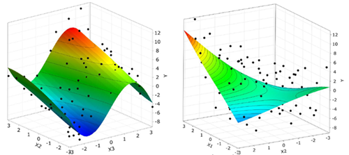

This function has several local and one dominant global minimum.

This tutorial demonstrates how to do the following:
Use the parameter and response definition from the sensitivity analysis
Specify the optimization criteria
Perform optimization on the Metamodel of Optimal Prognosis (MOP) from the sensitivity analysis
Perform direct optimization in full parameter space using the Adaptive Metamodel of Optimal Prognosis (AMOP)
You must complete the Sensitivity Analysis of a Coupled Function tutorial before starting this one.
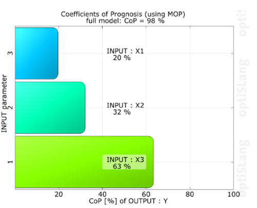
The sensitivity analysis indicates, that only X1 , X2 and X3 are important variables for a global optimization.
Optimization is performed in the reduced design space.

To set up and run the tutorial, perform the following steps:
Start optiSLang.
From the Start screen, click .

Browse to the location of the sensitivity analysis project you created in the previous tutorial and click .
Right-click the Sensitivity system and select from the context menu.
Repeat step 4 for the AMOP system.
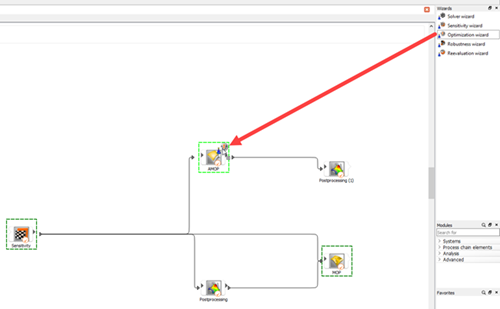
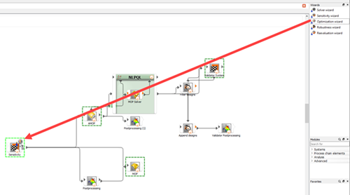
From the Wizards pane, drag the Optimization to the AMOP node and let it drop.
Do not adjust the values in the Parametrize Inputs table.
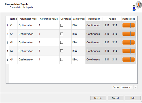
Click .
To define Y as a minimization objective, drag the row from the Responses table to the Objective Minimize icon and let it drop.
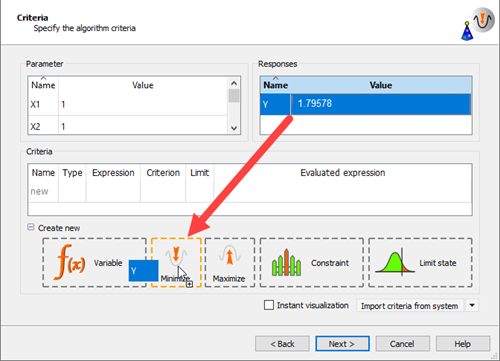
The new criterion is displayed in the Criteria table.
Click .
Click .
Do not adjust the current optimization method settings.
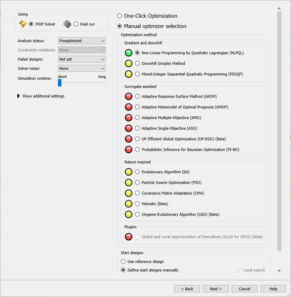
The gradient based NLPQL is recommended. Start designs can be selected manually.
Click .
Click .
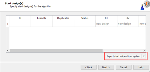
In the Select system pane, select AMOP.
In the Select designs to import pane, click the heading of the Y column to sort the data by response values.
Select the design at the top of the list and click .
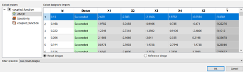
The selected design is added to the Start design(s) table.
Click .
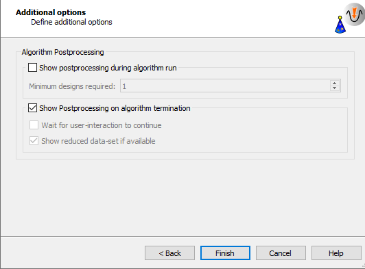
Leave the additional optional settings at the default and click .
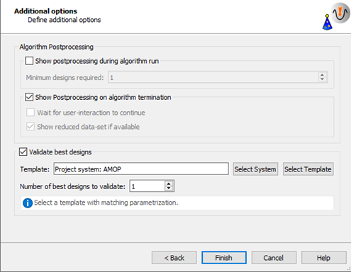
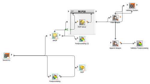
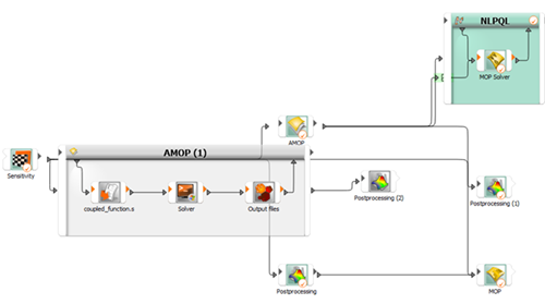
The optimization and validation flow is added to the Scenery pane.
To save the project, click
 .
.To run the project, click
 .
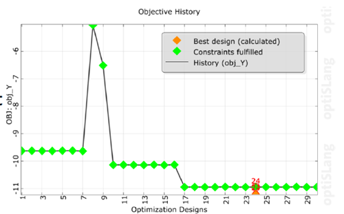
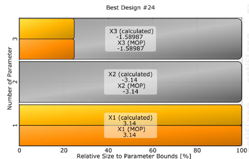
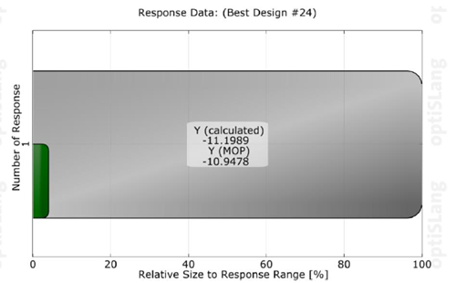
.The optimizer should converge in a few iteration steps. The response and objective of the best design are verified with the solver. Due to local approximation errors the estimated response value may differ from the solver result. Validation of the best design is necessary.
From the Wizards pane, drag the Optimization wizard to the Sensitivity node and let it drop.
Do not adjust the values in the Parametrize Inputs table.
Click .
To define Y as a minimization objective, drag the row from the Responses table to the Objective Minimize icon and let it drop.
The new criterion is displayed in the Criteria table.
Click .
Click .
Do not adjust the current optimization method settings.
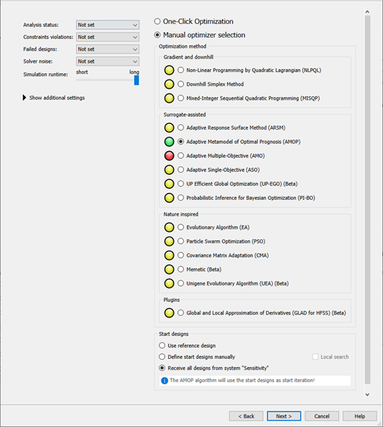
The Adaptive Metamodel of Optimal Prognosis (AMOP) is recommended. All previous designs are considered as start designs.
Click .
Leave the additional optional settings at the default and click .
The AMOP system is connected to the previous sensitivity system. The best design of the previous optimization is imported automatically.
Right-click the AMOP (1) system and select from the context menu.
Change the name to
AMOP_localand press Enter.
Double-click the AMOP_local system to open the settings.
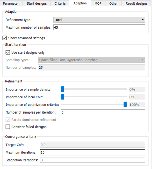
On the Adaption tab, select the Show advanced settings check box.
In the Maximum number of samples field, enter
45.Adjust the refinement sliders so the first two are at 0% and the Importance of optimization criteria slider is at 100%
In the Maximum iterations field, enter
10.
To save and close the settings, click .
To save the project, click
.To run the project, click
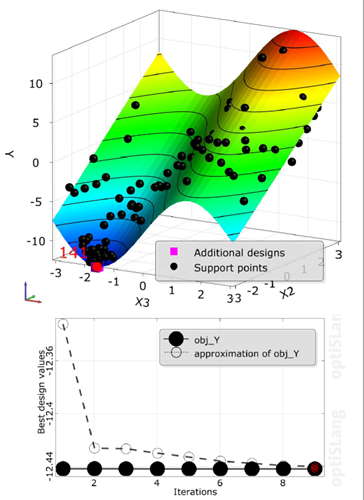
.The AMOP postprocessing is displayed. You can observe:
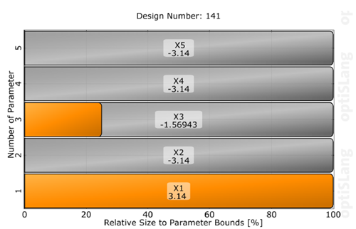
The AMOP with criteria refinement converges in a few iteration steps to the global optimum
Validation of best design is performed in every iteration
The history plot compares best design approximation and validation
The tutorial showed that:
Sensitivity analysis indicated three of five design variables as important
Optimization on the MOP lead to good optimal design in reduced space
Optimization in the full parameter space could be obtained efficiently by the AMOP
| Method | Best Objective | Solver Runs |
|---|---|---|
| Analytical solution | -12.4 | - |
| Initial design | 6.5 | 1 |
| Sensitivity analysis | -9.1 | 100 (300 with AMOP) |
| NLPQL on MOP | -11.2 | 1 |
| AMOP with local refinement | -12.4 | 100+45 |