

Examples are short descriptions of problems and links to files that you can explore without following a full tutorial.
The following examples are available:
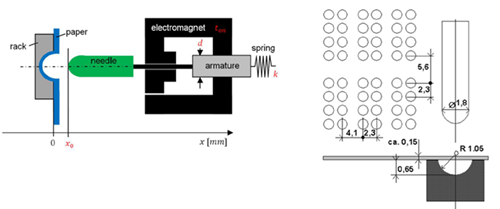
Each character consists of a 2x4 dot matrix. Four available needles need two stamps per character. 130 characters per second (260 stamps per second) are required. With a 10% safety margin, the maximum time for a full embossing cycle is 3.4 ms.
The optimization task is minimization of the cycle time with successful embossing.
For the example files, download the braille_printer_example zip file from here .
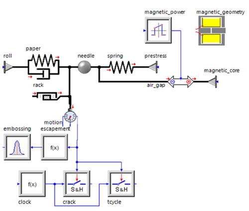
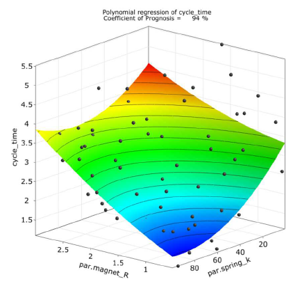
Sensitivity Analysis and Optimization
Perform a sensitivity analysis with the given parameter bounds:
Initial needle displacement: 0.15 – 2.0
Spring stiffness: 0.5 - 100
Diameter of magnetic armature: 5.0 – 15.0
Magnetic power-on time: 0.5 – 3.0
Responses are cycle time and embossing success.
The objective is to minimize cycle time.
The constraint function is embossing ≥ 1
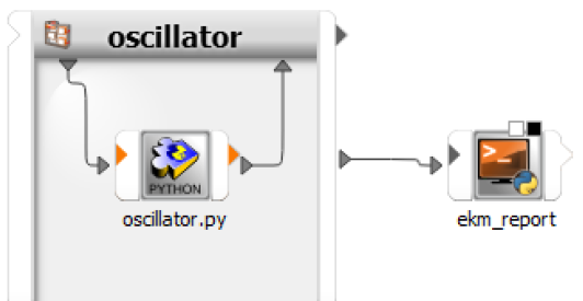
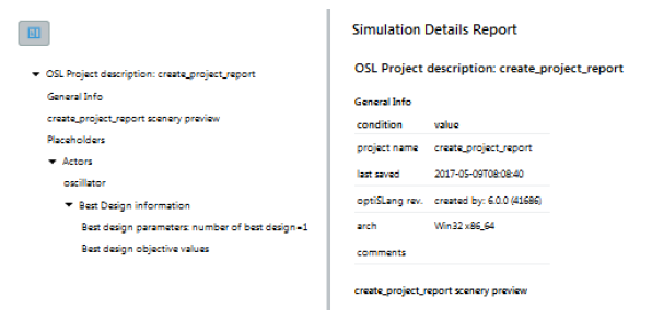
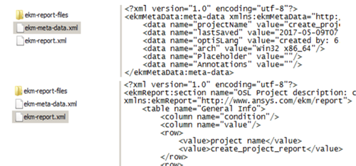
Generate a report of an optiSLang project into XML format.
For the example files, download the ekm_report_example zip file here .
You can generate the report two different ways:
Python process node: generate-ekm-report.py
Shell or batch script: generate-ekm-report.sh or generate-ekm-report.bat
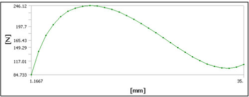
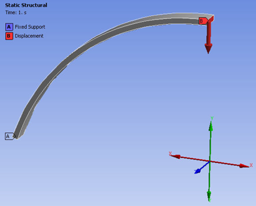
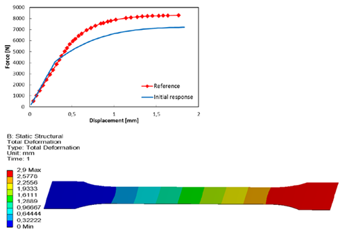
In this task, the input parameters should be adapted in such a way that a certain force-deflection curve is achieved.
The input parameters can vary within the following boundaries:
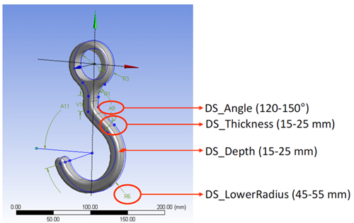
Thickness: 1 → 0.8 – 1.2
Radius: 35 → 32 – 37
Depth: 3 → 2.5 – 3.5
Height: 10 → 5 - 15
For the example files, download the force_displacement_example zip file here .
For this example, perform a sensitivity analysis using the global bounds of
 .
.
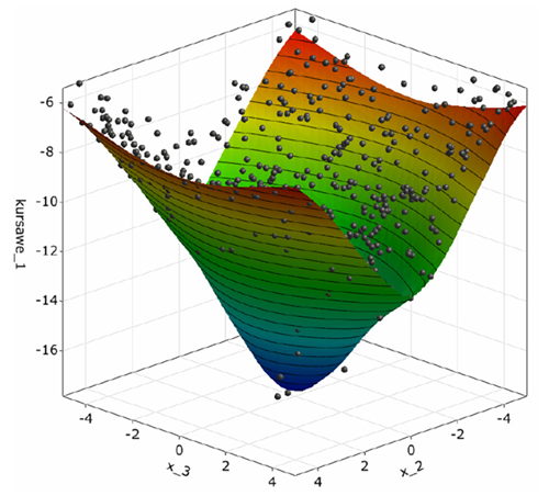
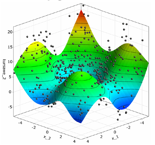
Perform multi-objective optimization by minimizing objective function one and two simultaneously.

For the example files, download the kursawe_example zip file here .
Objective function one has one dominant global optimum. Objective function two has four local optima.


Information about the optiSLang provided Python modules can be found here.
For the example files, download the python_examples zip file here .
Python Node
These scripts can be used to interact with nodes in the scenery.
modify_designs.py: Reads an optiSLang *.bin or *.omdb file and modifies a design container by adding responses and criteria
bestdesign_text.py: Writes the best design to an HTML file
csv_import.py: Reads a CSV file and writes content to an optiSLang monitoring database file
mop_2_file.py: Writes a CoP matrix and CoP filter model of MOP to a CSV file
print_monitoring_database.py: Writes an optiSLang *.bin or *.omdb file content to text file
filter_designs.py: Applies whitelist filtering of responses and criteria to designs from an optiSLang monitoring database file
export_fmu2.py: Exports a Metamodel of Optimal Prognosis (MOP) as a Functional Mock-Up Unit (FMU) 2.0 using the data from an optiSLang postprocessing file (*.omdb) and the optiSLang 3D Post-Processing Python module sos_package
Python Console
Copy the content of these files into the Python console of optiSLang or use it for batch mode.
[installation path]/tools/import/optislang3/convert.py : Creates a flow with TextInput, TextOutput and Solver nodes (converts a project from optiSLang3 to the current optiSLang version)
python_help.py: Prints help docstrings for actors
python_node.py: Inserts a Python node with custom script source to set up a parametric workflow
optimizer_settings.py: Modifies optimizer settings
sensitivity_settings.py: Modifies sensitivity settings
arsm_ten_bar_truss.py: Sets up an ARSM flow for the ten bar truss example
simple_calculator.py: Sets up a simple calculator node chain
ten_bar_truss_lc2.py: Modifies flow created by arsm_ten_bar_truss.py (adds load case 2)
ten_bar_modify_parameters.py: Modifies flow created by arsm_ten_bar_truss.ey (changes bounds)
ansys_workbench_ten_bar_truss.py: Creates a project with a Workbench node using the ten_bar_apdl example
ansys_workbench_portscan.py: Scans the port range used for communication with Workbench
extract_best_designs.py: Creates an *.omdb file with best designs
oscillator_system_python.py: Creates a parametric system for the oscillator Python example
oscillator _sensitivity_mop.py: Creates a sensitivity flow for the oscillator Python example
oscillator_optimization_on_mop.py: Adds an optimization on a MOP flow for the oscillator Python example
oscillator_optimization_ea.py: Creates an optimization using an EA flow for the oscillator Python example
oscillator_robustness_arsm.py: Creates a robustness flow for the oscillator Python example
omdb_reevaluate.py: Creates a reevaluation system to extract designs from the *.omdb file
Python Postprocessing
add_custom_data_plot.py: Create different plots (Line, Grid, Bar plot) of customized data
animate_models.py: Animation of metamodels
approximation_monitoring_export.py: Create and export approximation plots
InitializePostprocessingFromTextFileWithSettings.py: Loads a Statistics view directly from a CSV file and settings provided in the Python file.
Sensitivity_design_data.csv included in the example files.
InitializePostprocessingFromTextFileWithSettingsFile.py: Loads a Statistics view directly from a CSV file and JSON settings file.
Sensitivity_design_data.csv and Sensitivity_design_data.json included in the example files.
show_image.py: Show an user defined image
signal_plot.py: Extension of signal plot for oscillator example
traffic_light_plot.py: Extension of traffic light plot for ten bar truss example
optiSLang as a Server
get_basic_info_local.py: Connect to a local optiSLang server and print basic information
get_basic_info.py: Connect to a remote optiSLang plain TCP server and print basic information
get_basic_info_encrypted.py: Connect to a remote optiSLang SSL server and print basic information
get_basic_info_encrypted_password_protected.py: Connect to a remote, password protected optiSLang SSL server and print basic information
get_basic_info_zmq.py: Connect to a remote optiSLang ZeroMQ server and print basic information
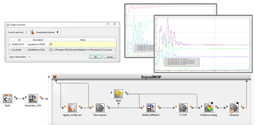
This example creates an automatic F-MOP analysis and generates a plot.
For the example files, download the signalmop_example zip file here .
For the example files, download the spring_steel_example zip file here .
Simulation Model
Identification of the material parameters to optimally fit the force-displacement curve to the following measurements:

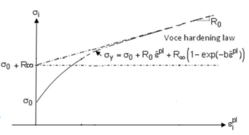
Unknown material parameters for nonlinear isotropic hardening (nliso):
Young´s modulus
Yield stress σ0
Linear hardening coefficient R 0
Exponential hardening coefficient R ∞
Exponential saturation parameter b
Simulation with Reference Parameters
Solver Chain
Simulation results in a force-displacement signal. The reference signal is taken from a text file. The sum of squares is calculated with the calculator.
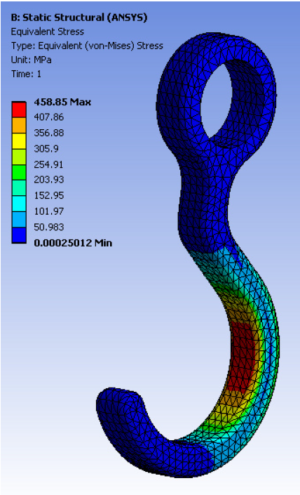
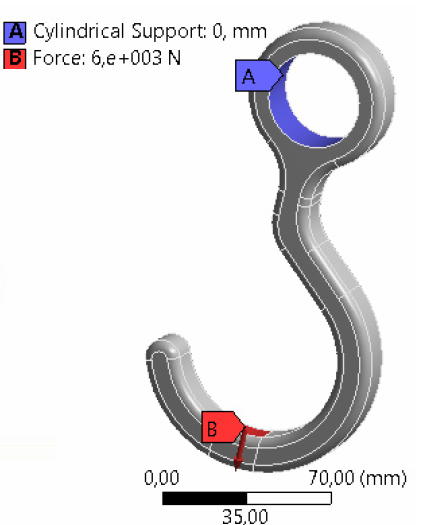
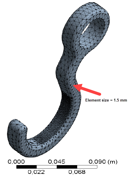
This example is to optimize the hook so that the v.-Mises stress does not exceed 300 MPa, the mass is as minimal as possible, and for certain geometry parameters to be in predefined bounds.
For the example files, download the hook_example zip file here .
Design Parameters using DesignModeler
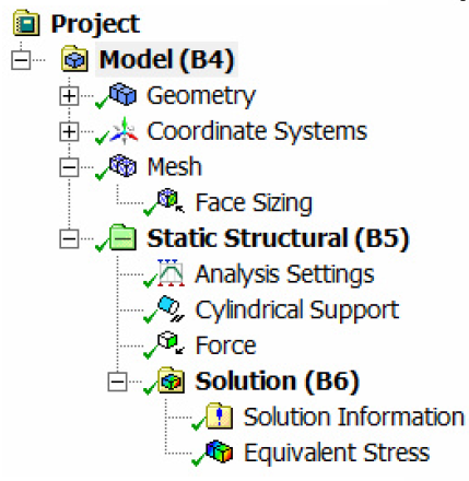
Boundary Conditions using Mechanical
Force is 6000 N. Cylindrical support, tangential direction is free.
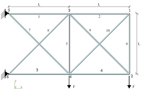
For the example files, download the ten_bar_truss_example zip file here .
Ten Bar Truss Structure
Load parameters: 
Material parameters: 
Element length: L = 360 in
Responses from linear finite element analysis are:
Mass
Displacement from loading points
Stresses for each element
Description
Analysis using the following global bounds: 
The goal is to minimize mass: 
Constraint: 
Robustness analysis at the deterministic optimum using normally distributed random
variables: 
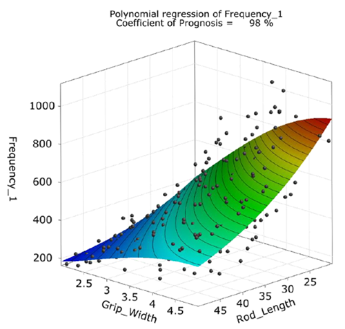
For the example files, download the tuning_fork_example zip file here .
Tuning Fork Design
A modal analysis of a tuning fork with fixed support and undamped oscillation is performed within Mechanical APDL.
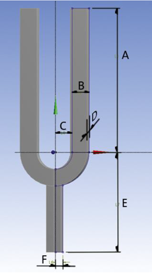
| A | Rod_Length | 20-50 mm |
| B | Rod_Width | 2-5 mm |
| C | Radius | 7-10 mm |
| D | Depth | 2-5 mm |
| E | Grip_Length | 15-30 mm |
| F | Grip_Width | 2-5 mm |
Optimization Task
Optimize the tuning fork to obtain:
1st Eigen-frequency = 440 Hz
2nd Eigen-frequency = 880 Hz
3rd Eigen-frequency = 1320 Hz
Minimum mass

Sensitivity Analysis and Optimization
Perform a sensitivity analysis with the given parameter bounds:
Rod length ∈ [20, 50 mm]
Rod width ∈ [2, 5 mm]
Radius ∈ [7, 10 mm]
Depth ∈ [2, 5 mm]
Grip length ∈ [15, 30 mm]
Grip width ∈ [2, 5 mm]
The objective function is the sum of squared errors of the target frequencies and the mass:

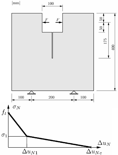
For the example files, download the wedge_splitting_example zip file here .
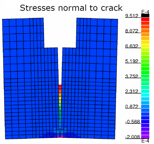
Simulation Model
2D linear elastic finite element model with a predefined crack. Bilinear softening for crack interface elements.
Unknown constitutive parameters:
Young’s modulus E
Poisson’s ratio

Tensile strength f t
Fracture energy G f
Shape parameters


Simulation with Reference Parameters
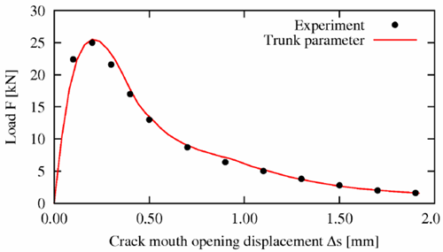
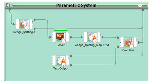
Solver Chain
Simulation results in a force-displacement signal. The reference signal is taken from a text file. The sum of squares is calculated with the calculator.
Calibration
Identification of the elasticity and fracture parameters to optimally fit the reference force-displacement function.
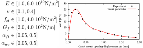
Objective function is the sum of squared errors between the reference and the calculated force displacement function values.
