This example demonstrates a workflow for applying the true geometry of a scanned compressor wheel as obtained from a 3D laser scan to Ansys Mechanical with minimum effort. Further, the technology can be used to generate new virtual geometries (for Monte Carlo-like studies) that are very close to the variation patterns and statistics as found in the measurements.
Note: A CAD0 reference geometry is usually a “perfectly” modelled geometry with no imperfections, in contrast to a laser-scanned real-world geometry.
Workflow Benefits
The workflow described in this example provides these benefits:
Easily maps the geometric measurements given in an STL file to a CAD0 reference geometry, allowing you to work on the FEM mesh, which is meshed only once, rather than on the CAD model
Can be automated
Applies and maps measurements onto the CAD0 FEM mesh and morphs the mesh accordingly
Creates a statistical shape model that auto-parametrizes the geometric variations as found in the measurements
Helps to analyze the statistical properties of the geometric variations
Helps to analyze the influence of the geometric variations onto the structural performance
Helps to do a sensitivity analysis identifying the importance of geometric imperfections compared with other scatter variables in robustness analysis
Workflow Applications
The workflow can be used in scenarios for:
Statistically analyzing the influence of geometry variations on fatigue behavior, lifetime, quality, structural performance, efficiency, and more, to assess the robustness and sensitivity of the structure
Bringing together CAD0 models and geometric measurements such as those seen in production tolerances, wear, design for manufacturing, and more
Identifying allowed tolerance windows to improve quality control after manufacturing
Analyzing sensitive structural components like compressor wheels, machine housings, molding parts, and more
This example starts with a measurement after manufacturing (an already preprocessed STL file) and an Ansys Workbench project containing the structural analysis of a compressor wheel for the CAD0 geometry.
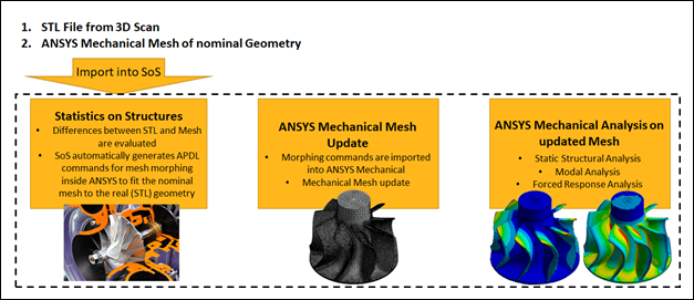
A summary follows of the solution steps for performing uncertainty quantification of the compressor wheel based on measured geometries:
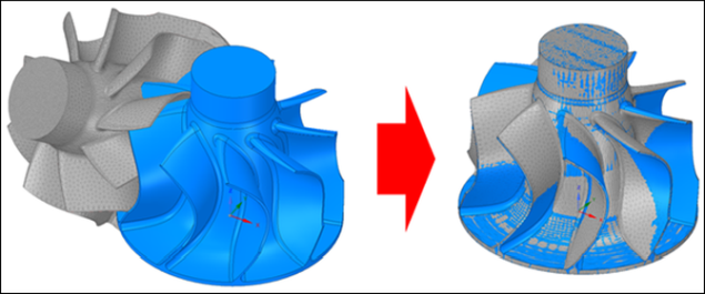
Use 3D scan data of models to represent the actual imperfect shape.
Prepare a mesh of the nominal CAD geometry in Ansys Mechanical.
Load both the 3D scan data and the mesh into oSP3D and perform deviation evaluation and morphing export to Mechanical.
Morph the mesh inside Mechanical to represent the imperfect geometry for simulation.
This image shows the workflow:
To prepare the mesh of the nominal CAD geometry:
In Ansys Workbench, open the archive file named TurbineWheel.wbpz in
oSP3D_examples\ansys\turbine.Rename the project to TurbineWheel and save it as a project file in the same folder.
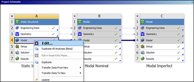
In the Static Structural system named Static Imperfect, right-click the Model cell and select to start Ansys Mechanical.
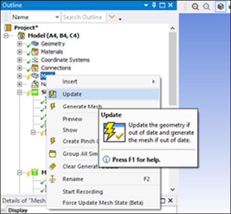
In the project tree, right-click Mesh and select , either keeping the settings as they are or changing them per your preference.
In the project tree under Named Selections, look at those that have been predefined and optionally define any additional faces that you want to morph.
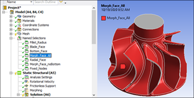
You can define as many faces to morph as you want, but they must be part of one named selection because you can select only one named selection inside oSP3D.
Additionally, you want to define a named selection with nodes that should be fixed later in oSP3D. This must be a set of nodes that is not part of the node set that will be morphed. In this example, the named selection Fixed_Nodes already exists.
In the project tree, select Static Structural and either keep the boundary conditions and loads as they are or change them per your preference.
In the project tree, select Morphing.
In the code snippet, change the value for the variable
prep_meshto1.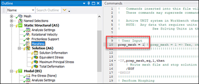
Note: Changing
prep_meshto1triggers Mechanical to stop before it starts solving the model. Thus, Mechanical will produce only the Ansys input file (ds.dat), which contains all finite element data of the model. This ds.dat file will later be used to read the FE data into oSP3D.Change the solver units to millimeters and tons:
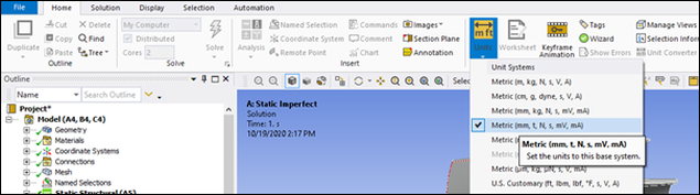
Caution: Because the STL file is prepared in millimeter units, you must change the units in Mechanical to millimeter units before solving. If the scan and the mesh are not of the same size, the morphing will fail.
In the project tree, right-click Solution for this Static Structural system and select .
Mechanical starts solving and will stop with an error, which is fine, because no simulation was run. Your objective is only to produce the mesh file (ds.dat) with all the finite element information and named selections for import into oSP3D.
Note: Aligning the STL file with the CAD geometry file is not required to continue this example. However, you must align "fresh" scan data with an STL file. For more information, see Aligning the STL and CAD Geometry Files in SpaceClaim.
As indicated in the following image, once you have prepared the mesh data file (ds.data) and aligned STL scan file, you can import them into oSP3D.
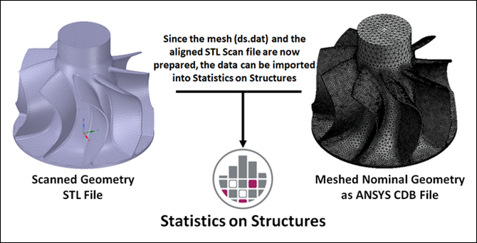
To import these files into oSP3D:
Start a new oSP3D project, choosing the ds.data file that was created in
oSP3D_examplesansys\turbine as the reference mesh and naming the projectTurbineWheel.Set the reference named selection:
Select > > .
In the window that opens, make these selections:
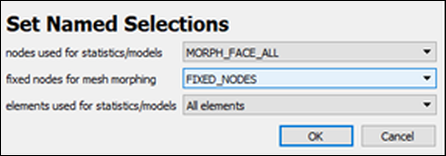
Import the STL file:
Select > > .
In the Import Designs window, click Add file and open the STL file in your working directory (TurbineWheel_Scan.stl).
oSP3D reads the STL file and gives you a summary of the imported data:
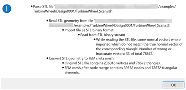
Click .
In the Import designs window, the file TurbineWheel_Scan.stl is shown in the list of files to parse.
For Mesh mapper, select Incompatible and then click Settings.
In the Configure incompatible mesh mapper window, set Maximum search distance to a reasonable value that corresponds to the maximum deviation observed between the scan and the nominal CAD geometry.
For this example, set the value to 1.0 mm.
Click .
In the Data to import area of the Import designs window, select only the CoorDeviationNormal check box in the Imported ident column.
Click .
Leave the settings in the Design directories area as they are.
Click Finish.
oSP3D imports the scan and evaluates the deviations compared to the nominal mesh. This takes about three minutes.
Save the oSP3D database:
Select > .
In the window that opens, enter
mophing.sdbas the file name and click .
Export the morphing script:
Select > > .
In the Export Designs window, set the path to your reference design to your working directory (
oSP3D_examples\TurbineWheel).Click .
In the window that opens, enter
morphingas the file name and click .In the Export designs window, for the export item Normal coordinate deviation, select CoorDeviationNormal in the Quantity ident column.
Under the list of items to export, select the Use mesh smoothening check box.
Click .
Leave the settings in the Design directories area as they are.
Click Finish.
oSP3D exports the morphing script. This takes about 10 minutes.
To use the exported morphing script in a Mechanical solve:
In the project tree, select Morphing.
In the code snippet, change the value for the variable
prep_meshto0.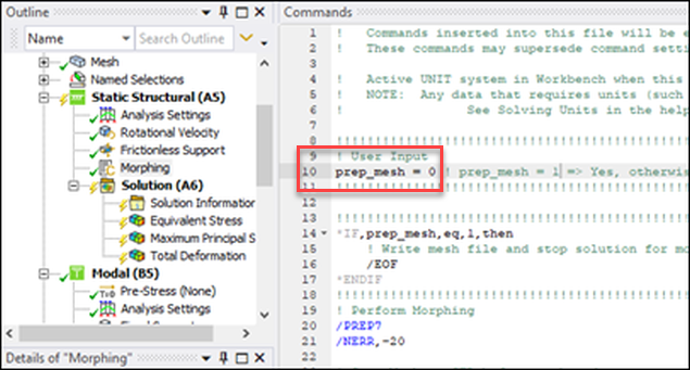
In the project tree, right-click Solution for this Static Structural system and select .
In the project tree, select Solution for this Static Structural system and, in the Details view, set Mesh Source (Beta) to Result File.
Visualize and observe the results.
The following results are for static with 75000 RPM.
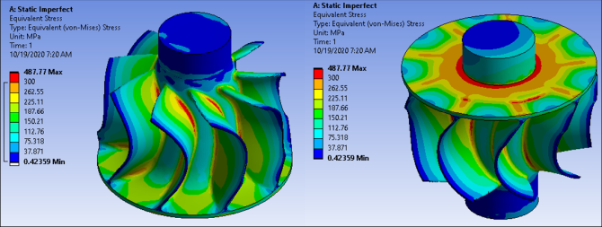
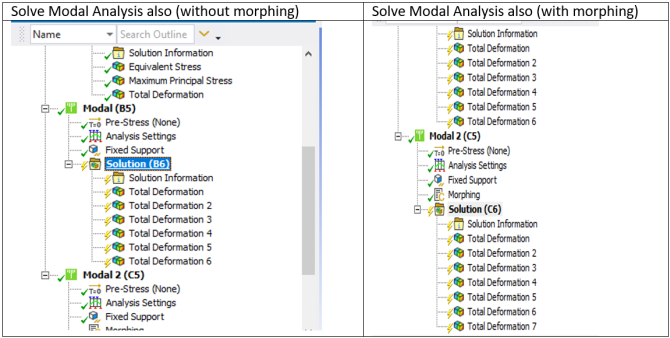
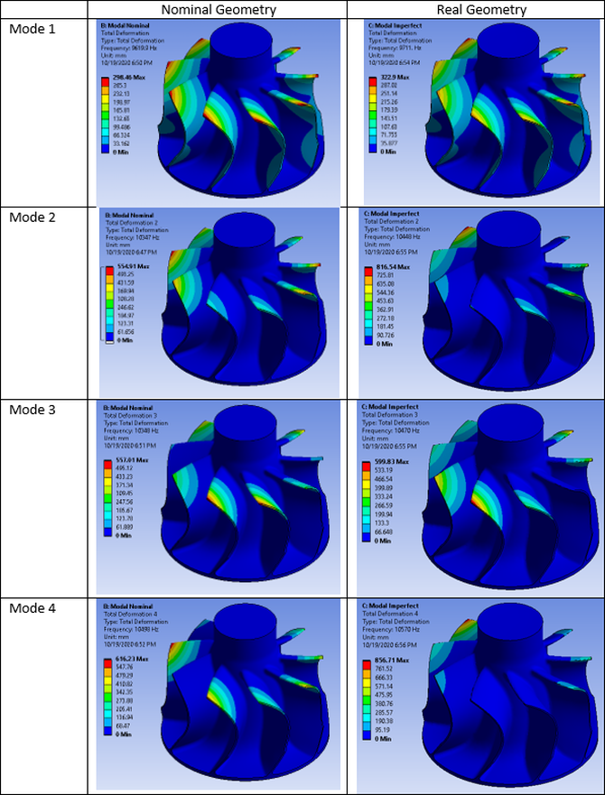
As expected, the compressor blades are longer, leading to lowered eigenfrequencies.
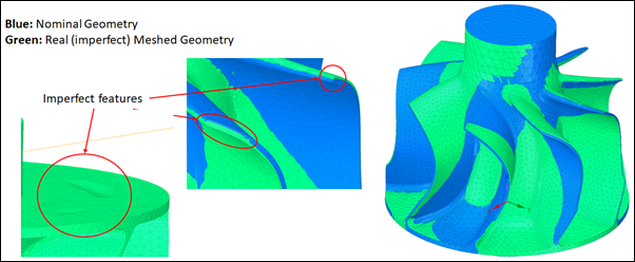
To observe differences between the nominal geometry and real geometry:
Go to the Ansys Workbench folder path: …\TurbineWheel_files\dp0\SYS-1\MECH\
In this folder, two STL files (nominal_geometry.stl and real_geometry.stl) were saved after solving the Static Structural system using the writestl.mac APDL macro.
Open SpaceClaim and import these files.
Observe differences of the geometry before and after morphing.
Additionally, import the original STL file (TurbineWheel_Scan.stl) that is in your working directory (location of the Workbench project).
In the Measure ribbon, click Deviations.
In the project tree, under > , select > to be the source and then press and hold down the Ctrl key and select > .
Deviations are shown.
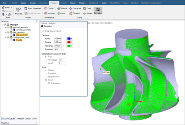
In the Options Analysis window, change the evaluated tolerances as preferred.
To align an STL file with 'fresh' data to a CAD geometry file in SpaceClaim:
Start SpaceClaim and open the STL scan file (TurbineWheel_Scan.stl).
Observe the facet density and features of the STL file.
For this example, you want to keep the facet density as it is. The STL file has already been prepared to have the density needed to cover all features.
STL files with ‘fresh’ scan data must be aligned to fit the position of the nominal CAD geometry. The number of facets must be dramatically reduced, to have fewer than 100k facets if possible. To reduce the number of facets on 'fresh' scan data, on the Facets ribbon, you would click Reduce.
Align the scan with the nominal CAD geometry that you used for meshing inside Ansys Mechanical.
The geometry in this example is already perfectly aligned.