Random variables are scalar quantities which may be represented by a set of discrete values, each having a specific probability, or by continuous variables defined in a given range. A continuous random variable X is described by the cumulative distribution function
 | (4–2) |
where P [X < x] is the probability that X is lower than a given value x.
|
|
|
Cumulative distribution function |
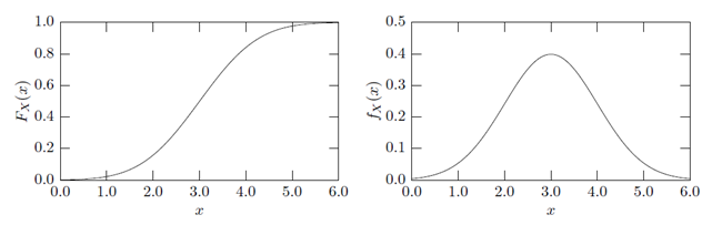


Equivalent to the cumulative distribution function often the probability density function, which is the derivative of the cumulative distribution function, is utilized
 | (4–3) |
In Figure 4.2: Cumulative Distribution Function and Probably Density Function, the cumulative distribution function and the probability density function of a continuous random variable are shown exemplary.
Based on the density function, stochastic moments have been introduced, see for example (Bucher 2009). The first, absolute moment of a random variable X is its mean value
 | (4–4) |
where E[·] is the expected value. The second, central moment of a random variable is its variance
 | (4–5) |
Mean value and variance (or standard deviation  ) are typically used to describe the variation of a random
variable. However, even the shape of the distribution function may have a
significant influence on the results of a stochastic analysis. Specific distribution
types have been proposed during the last centuries. The most famous is the normal
(Gaussian) distribution. Other common distribution types are e.g. uniform,
log-normal, exponential, Gumbel, and Weibull distributions. In optiSLang a large
number of well-known distribution types is available. The probability density
functions and properties are given in Distribution Types.
Further details on distribution types of random variables can be found for example
in (Montgomery and Runger 2003) and (Bucher 2009).
) are typically used to describe the variation of a random
variable. However, even the shape of the distribution function may have a
significant influence on the results of a stochastic analysis. Specific distribution
types have been proposed during the last centuries. The most famous is the normal
(Gaussian) distribution. Other common distribution types are e.g. uniform,
log-normal, exponential, Gumbel, and Weibull distributions. In optiSLang a large
number of well-known distribution types is available. The probability density
functions and properties are given in Distribution Types.
Further details on distribution types of random variables can be found for example
in (Montgomery and Runger 2003) and (Bucher 2009).
In order to perform a robustness analysis, optiSLang requires the definition of distribution types including mean value and standard deviation for all random input variables. Since the stochastic properties of the inputs have a significant influence on the results of a robustness analysis, the user is requested to consider as much information as possible for this purpose. If measurements should be considered, the statistic post processing of optiSLang can be used to estimate the stochastic moments and to find a suitable distribution type.
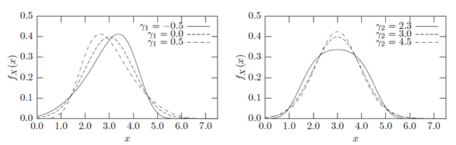
Additionally to mean value and standard deviation often higher order moments of
random model responses and even of random inputs are of interest. Skewness  and kurtosis
  are the standardized third and fourth moments of a random
variable
are the standardized third and fourth moments of a random
variable
 | (4–6) |
They provide a description of the shape of a random variable density function in addition to mean value and standard deviation. For example, for symmetric density functions the skewness is always zero and for the normal distribution the kurtosis is equal to three. In Figure 4.3: Density Functions with Corresponding Skewness and Kurtosis Values, several density functions are shown together with corresponding skewness and kurtosis values.