As demonstrated in the previous section, the prediction quality of an approximation model may be improved if unimportant variables are removed from the model. This idea is adopted in the Metamodel of Optimal Prognosis (MOP) proposed in (Most and Will 2008) which is based on the search for the optimal input variable set and the most appropriate approximation model (polynomial or MLS with linear or quadratic basis). Due to the model independence and objectivity of the CoP measure, it is well suited to compare the different models in the different subspaces.
Figure 2.8: CoP Values of Different Input Variable Combinations and Approximation Methods Obtained with the Analytical Nonlinear Function
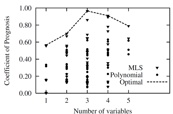
In Figure 2.8: CoP Values of Different Input Variable Combinations and Approximation Methods Obtained with the Analytical Nonlinear Function, the CoP values of all possible subspaces and all possible approximation models are shown for the analytical nonlinear function example. The figure indicates that there exists an optimal compromise between the available information, the support points and the model complexity i.e. the number of input variables. The MLS approximation by using only the three major important variables has a significantly higher CoP value than other combinations. However for more complex applications with many input variables it is necessary to test a huge number of approximation models. In order to decrease this effort, in (Most and Will 2008) advanced filter technologies are proposed, which reduce the number of necessary model tests. Nevertheless, a large number of inputs requires a very fast and reliable construction of the approximation model. For this reason polynomials and MLS are preferred due to their fast evaluation.
As a result of the MOP, we obtain an approximation model which contains the most important variables. Based on this meta-model, the total effect sensitivity indices, proposed in First Order and Total Effect Sensitivity Indices, are used to quantify the variable importance. The variance contribution of a single input variable is quantified by the product of the CoP and the total effect sensitivity index estimated from the approximation model
 | (2–18) |
Since interactions between the input variables can be represented by the MOP approach, they are considered automatically in the sensitivity indices. If the sum of the single indices is significantly larger as the total CoP value, such interaction terms have significant importance.
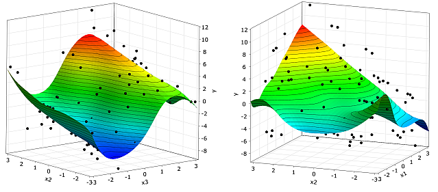
Additionally to the quantification of the variable importance, the MOP can be used to visualize the dependencies in 2D and 3D subspaces. This helps the designer to understand and to verify the solver model. In Figure 2.9: Subspace Plots, two subspace plots are shown for the MOP of the analytical test function. In the X2-X3 and X1- X2 subspace plots, the sinusoidal function behavior and the coupling term can be observed. Additional parametric studies, such as global optimization can also be directly performed on the MOP. Nevertheless, a single solver run should be used to verify the final result of such a parametric study or optimization.
|
|
|
X2-X3 and X1-X2 subspace plots of the MOP of the nonlinear analytical function given in Equation 2–12. |