


By definition, sensitivity analysis is the study of how the uncertainty in the output of a model can be apportioned, qualitatively or quantitatively, to different sources of variation in the input of a model (Saltelli et al. 2008). In order to quantify this contribution, variance based methods are very suitable. With these methods the proportion of the output variance, which is caused by an random input variable, is directly quantified.
Variance based sensitivity analysis is also very suitable as an optimization pre-processing tool. By representing continuous optimization variables by uniform distributions without variable interactions, variance based sensitivity analysis quantifies the contribution of the optimization variables to a possible improvement of the model responses. In contrast to local derivative based sensitivity methods, the variance based approach quantifies the contribution with respect to the defined variable ranges.
Unfortunately, sufficiently accurate variance based methods require huge numerical effort due to the large number of simulation runs. Therefore, often meta-models are used to represent the model responses by surrogate functions in terms of the model inputs. However, many meta-model approaches are available and it is often not clear which one is most suitable for which problem (Roos et al. 2007). Another disadvantage of meta-modeling is its limitation to a small number of input variables. Due to the so-called "curse of dimensionality" the approximation quality decreases for all meta-model types dramatically with increasing dimension. As a result, an enormous number of samples is necessary to represent high-dimensional problems with sufficient accuracy. In order to overcome these problems, we developed the Metamodel of Optimal Prognosis (Most and Will 2008). In this approach the optimal input variable subspace together with the optimal meta-model are determined with help of an objective and model independent quality measure, the Coefficient of Prognosis. In the following chapter the necessity of such a procedure is explained by discussing other existing methods for sensitivity analysis. After presenting the MOP concept in detail, the strength of this approach is clarified by a comparison with very common meta-model approaches such as Kriging and neural networks
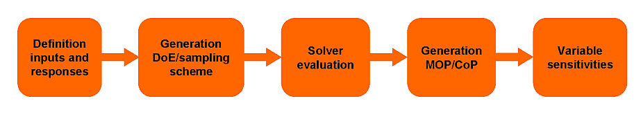
In Figure 2.1: Flowchart of optiSLang Sensitivity Analysis the general flow of an optiSLang sensitivity analyis is shown: after the definition of the design variables and model responses the design space is scanned by Design of Experiments or sampling methods. These samples are evaluated by the solver and for each design the model responses are determined. Approximation models are built for each model response and assessed regarding their quality. Finally variance based sensitivity indices are estimated by using the approximation models.