


This tutorial demonstrates using Steady-State and Transient Thermal analyses to investigate the temperatures caused by heat generated in chips on a circuit board.
| Analysis Type | Transient Thermal |
| Features Demonstrated | Linked analyses, attaching geometry, model manipulation, mesh method and sizing controls, constant and time-varying loads, time-history results, result probes, charts |
| Licenses Required | Ansys Mechanical Premium/Enterprise/Enterprise PrepPost |
| Help Resources | Steady-State Thermal Analysis, Transient Thermal Analysis Type |
| Tutorial Files | BoardWithChips.x_t |
This tutorial guides you through the following topics:
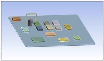
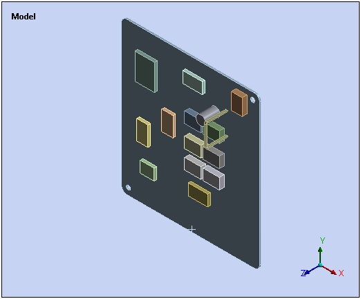
The circuit board shown below includes three chips that produce heat during normal operation. One chip stays energized as long as power is applied to the board, and two others energize and de-energize periodically at different times and for different durations. A Steady-State Thermal analysis and Transient Thermal analysis are used to study the resulting temperatures caused by the heat developed in these chips.
Establish a transient thermal analysis that is linked to a steady-state thermal analysis.
Start Ansys Workbench.
From the Toolbox, drag a Steady-State Thermal system onto the Project Schematic.
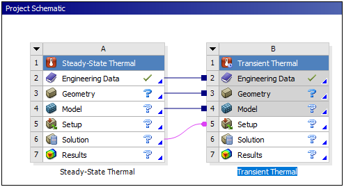
From the Toolbox, drag a Transient Thermal system onto the Steady-State Thermal system such that cells 2, 3, 4, and 6 are highlighted in red.
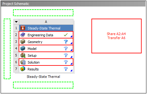
Release the mouse button to define the linked analysis system.
Attach Geometry
In the Steady-State Thermal schematic, right-click the Geometry cell, and then choose Import Geometry.
Browse to open the file BoardWithChips.x_t. This file is available here on the Ansys customer site.
Prepare the Analysis System
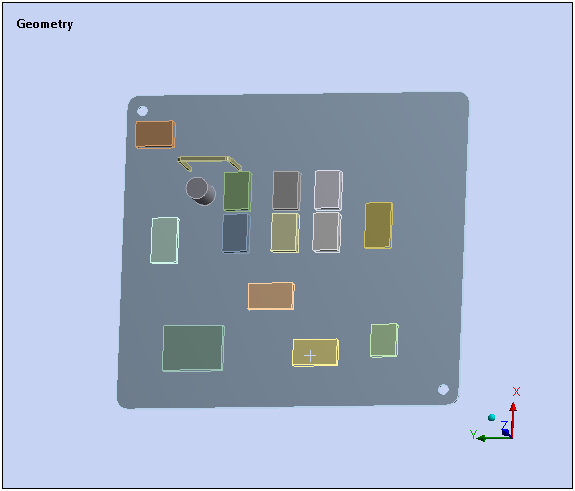
In the Steady-State Thermal schematic, right-click the Model cell, and then choose Edit. The Mechanical Application opens and displays the model.
For convenience, use the toolbar button to manipulate the model so it displays as shown below.
Note: You can perform the same model manipulations by holding down the mouse wheel or middle button while dragging the mouse.
From the Tools group on the Home tab, open the Units drop-down menu and select .
Setting a specific mesh method control and mesh sizing controls will ensure a good quality mesh.
Mesh Method:
Right-click the Mesh object and select > .
Select all bodies by right-clicking in the Geometry window and selecting . Click the button for the Geometry property in the Details view.
Set the Method property to Multi Zone.
Mesh Body Sizing – Board Components:
Right-click the Mesh object and select > .
Select all bodies except the board by first enabling the selection toolbar button, then holding the Ctrl keyboard button and clicking on the 15 individual bodies. Click the button for the Geometry property in the Details view when you are done selecting the bodies.
Change Element Size from Default to 0.0009 m.
Mesh Body Sizing – Board:
Right-click the Mesh object and select > .
Select the board only (1 Body) and change Element Size from Default to 0.002 m.
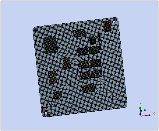
Generate Mesh:
Right-click the Mesh object and select Generate Mesh.
The chip on the board that is constantly energized represents an internal heat generation load of 5e7 W/m3.
Select the chip shown below by first enabling the selection toolbar button, then clicking on the chip.
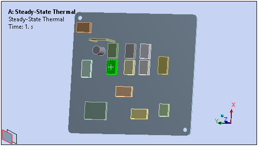
Right-click the Steady-State Thermal object and select > .
Enter
5e7in the Magnitude property and press Enter.General items to note:
The applied loads are shown using color coded labels in the graphics.
Time is used even in a steady-state thermal analysis.
The default end time of the analysis is 1 second.
In a steady-state thermal analysis, the loads are ramped from zero. You can edit the table of load vs. time to modify the load behavior.
You can also type in expressions that are functions of time for loads.
The entire circuit board is subjected to a convection load representing Stagnant Air - Simplified Case.
Select all bodies by right-clicking in the Geometry window and selecting .
Choose Convection from the Environment toolbar.
Import temperature dependent convection coefficient and choose Stagnant Air - Simplified Case. Note that the Ambient Temperature defaults to 22oC.
Click the flyout menu in the Film Coefficient field and choose Import Temperature Dependent (adjacent to the thermometer icon).
Click the radio button for Stagnant Air - Simplified Case, then click .
Prepare for a temperature result.
The resulting temperature of the entire model will be reviewed.
Right-click the Solution object and select > > .
Solve the steady-state thermal analysis.
Select the Solve option.
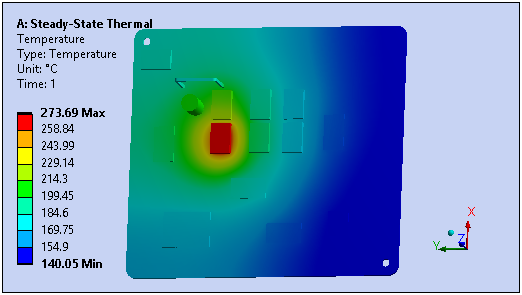
Review the temperature result.
Select the Temperature object.
You have completed the steady-state thermal analysis, which is the first part of the overall objective for this tutorial. You will perform the transient thermal analysis in the remaining steps.
Items to note in preparation for the transient thermal analysis:
If you highlight Initial Temperature object under the Transient Thermal object, you will notice in the Details view the read only displays of Initial Temperature and Initial Temperature Environment. In general, the initial temperature can be:
Uniform Temperature: where you specify a temperature for all bodies in the structure at time = 0, or
Non-Uniform Temperature: (as in this example) where you import the temperature specification at time = 0 from a steady-state analysis.
The initial temperature environment is from the steady-state thermal analysis that you just performed. By default the last set of results from the steady-state analysis will be used as the initial condition. You can specify a different set (different time point) if multiple result sets are available.
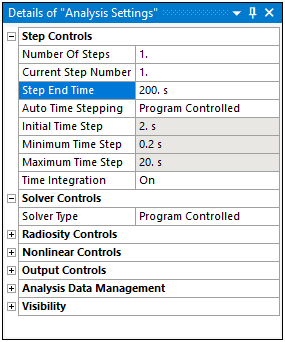
Specify a time duration for the transient analysis.
A time duration of the transient study will be 200 seconds.
Under Transient Thermal analysis, select the Analysis Settings object and enter 200 in the Step End Time property. Accept the default initial, maximum, and minimum time step controls for this analysis.
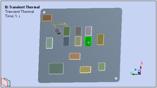
A chip on the board is energized between 20 and 40 seconds and represents an internal heat generation load of 5e7 W/m3 during this period.
Select the chip shown below using Body selection filter.
Right-click the Transient Thermal object and select > .
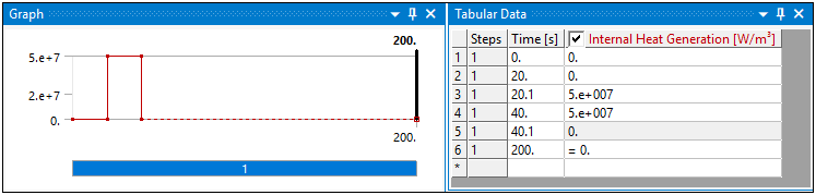
Specify the Magnitude property as . Enter the following data in the Tabular Data window:
Time = 0; Internal Heat Generation = 0
Note: Enter each of the following sets of data in the row beneath the end time of 200 s.
Time = 20; Internal Heat Generation = 0
Time = 20.1; Internal Heat Generation = 5e7
Time = 40; Internal Heat Generation = 5e7
Time = 40.1; Internal Heat Generation = 0
The Graph window reflects the data that you entered.
General items to note:
Loads can be specified as one of three types:
Constant: remains constant throughout the time history of the transient.
Tabular (Time): (as in this example) define a table of load vs. time.
Function: enter a function such as "=10*sin(time)" to define a variation of load with respect to time. The function definition requires you to start with a ‘=‘ as the first character.
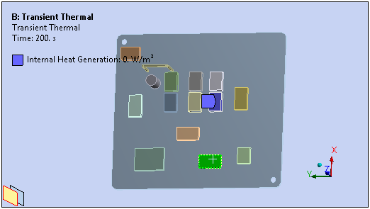
Apply internal heat generation to simulate on/off switching on second chip.
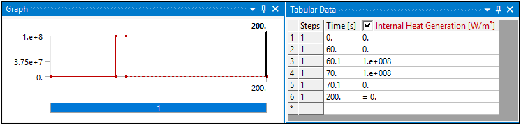
Another chip on the board is energized between 60 and 70 seconds and represents an internal heat generation load of 1e8 W/m3 during this period.
Select the chip shown below using the selection filter.
Right-click the Transient Thermal object and select > .
Specify the Magnitude property as . Enter the following data in the Tabular Data window:
Time = 0; Internal Heat Generation = 0
Note: Enter each of the following sets of data in the row beneath the end time of 200 s.
Time = 60; Internal Heat Generation = 0
Time = 60.1; Internal Heat Generation = 1e8
Time = 70; Internal Heat Generation = 1e8
Time = 70.1; Internal Heat Generation = 0
The Graph window reflects the data that you entered.
Prepare for a temperature result.
The resulting temperature of the entire model will be reviewed.
Right-click the Solution object and select > > .
Solve the transient thermal analysis.
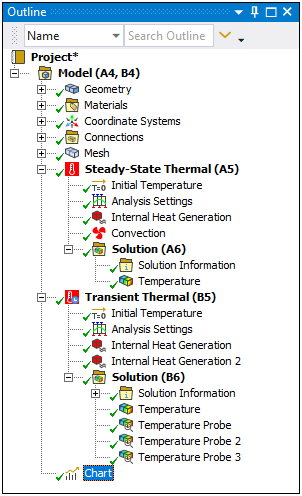
Right-click the Solution object and select . The solution is complete when green checks are displayed next to all of the objects. You can ignore the Warning message and click the Graph tab.
Review the time history of the temperature result for the entire model.
Highlight the Temperature object. The time history of the temperature result for the entire model is evaluated and displayed.
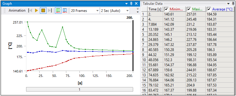
For the selected result, you can:
View the Minimum, Maximum, and Average values of the temperature result in the Tabular Data window.
Review the result value of a particular time point by selecting the desired point in the Graph window or right-clicking a point and selecting the Retrieve this Result option. You can also make selections in the Tabular Data window to retrieve result values.
Animate the solution.
Review the time history of the temperature result for each of the chips.
Temperature probes are used to obtain temperatures at specific locations on the model.
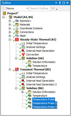
Right-click the Solution object and select > > .
Select the chip to which internal heat generation load was applied in the Steady State analysis and click the button in the Details view.
Follow the same procedure to insert two more probes for the two chips with internal heat generations in the transient thermal analysis.
Right-click the Solution object or Temperature Probe object and select .
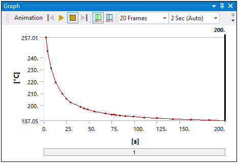
Select the three Temperature Probes and select the option in the Insert group of the Result Context tab. A Chart object is added to the tree.
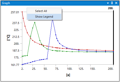
Right-click in the white space outside the chart in the Graph window and choose Show Legend.
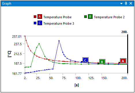
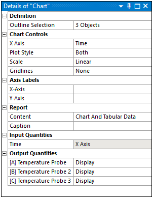
In the Details view, you can change the X Axis variable as well as selectively omit data from being displayed.
You have completed the second part of this tutorial, the transient thermal analysis.
Congratulations! You have completed the tutorial.