VM-LSDYNA-EMAG-002

VM-LSDYNA-EMAG-002
Hollow Conducting Sphere in a Uniform Magnetic Field

Overview

Reference:	EMSON, C.R.I. (1990) Summary of results for hollow conducting sphere in uniform transiently varying magnetic field (problem 11). COMPEL—The International Journal for Computation and Mathematics in Electrical and Electronic Engineering, 9, (3), 191-203. Ren, Z. (1989, October) Private communication: Analytic solution for hollow sphere in uniform field with a step function time variation. Laboratoire de Genie Electrique de Paris, France.
Analysis Type(s):	Electromagnetism
Element Type(s):	Solid Elements ELFORM 1, Shell Elements ELFORM 2
Input Files:	Link to Input Files Download Page

Test Case

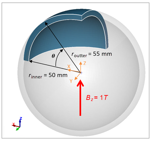
The TEAM 11 problem is a hollow conducting sphere, having an inner radius of 5cm and an outer radius of 5.5 cm. The sphere has a conductivity of 5.0 x 10E08 S/m, and a relative permeability of unity. A uniform magnetic field is incident (in the z-direction). At time t = 0, the field (initially zero) is switched to 1 Tesla instantaneously. The transient behavior of the field is to be modeled, including the nature of the induced eddy currents. The goal is to compute the magnetic field for different times and different positions as well as the current density at different angles.

Figure 168: Problem sketch and location of the origin and definition of the angle

Material Properties	Geometric Properties	Loading
r_inner = 50 mm	κ = 5.0∙10⁸ S/m	E_{z, initial} = 0T
r_outer = 55 mm	μ_r = 1	E_z_{(t = 0)} = 1T

Analysis Assumptions and Modeling Notes

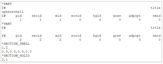
The LS-DYNA *EM_CONTROL card is set to 1 to activate the Eddy Current solver. The external magnetic field is applied using the *EM_EXTERNAL_FIELD card where the direction of the field and the load are specified.

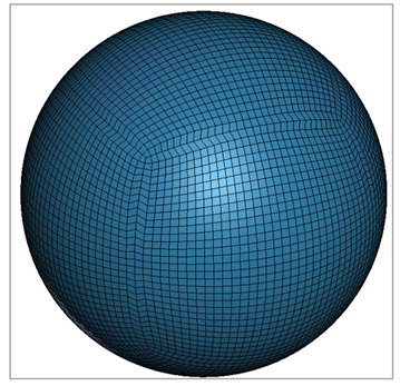
The mesh is formed by a solid mesh with element formulation 1 which is a constant stress solid element. A shell mesh is also created on top of the solid one with element formulation 2. This shell mesh is used by the BEM (Boundary Element Method) solver.

Figure 169: Model Mesh

Figure 170: Section cards in input deck

Results Comparison

The analytic solution is compared with LS-DYNA output. Simulation results are extracted from em_pointout.dat file. The origin is located at the center of the sphere and shown in Figure 168, as well as the angle.

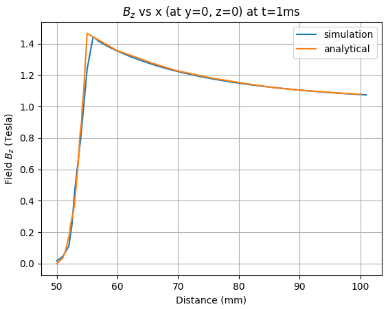
The error between the analytical solution and the simulation is presented in the following tables at several distances.

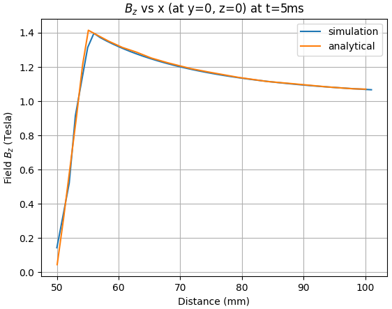
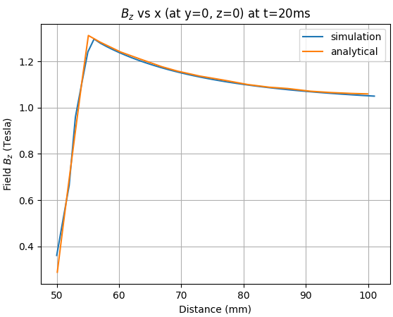
Table 4: z-Bfield for several x coordinates (at y = 0, z = 0) for 1 ms, 5 ms and 20 ms

Result	Target	LS-DYNA	Error (%)
z Field at t = 1 ms for x = 60 mm	1.34	1.35	1.32
z Field at t = 1 ms for x = 70 mm	1.21	1.22	1.25
z Field at t = 1 ms for x = 80 mm	1.17	1.15	1.66
z Field at t = 1 ms for x = 90 mm	1.11	1.10	0.68
z Field at t = 1 ms for x = 90 mm	1.11	1.10	0.68
z Field at t = 1 ms for x = 100 mm	1.08	1.08	0.50
z Field at t = 5 ms for x = 60 mm	1.33	1.32	1.00
z Field at t = 5 ms for x = 70 mm	1.21	1.20	0.53
z Field at t = 5 ms for x = 80 mm	1.13	1.13	0.66
z Field at t = 5 ms for x = 90 mm	1.09	1.09	0.15
z Field at t = 5 ms for x = 90 mm	1.09	1.09	0.15
z Field at t = 20 ms for x = 50 mm	1.07	1.07	0.25
z Field at t = 20 ms for x = 60 mm	1.26	1.24	1.84
z Field at t = 20 ms for x = 70 mm	1.15	1.15	0.27
z Field at t = 20 ms for x = 80 mm	1.11	1.10	0.81
z Field at t = 20 ms for x = 90 mm	1.08	1.07	0.58
z Field at t = 20 ms for x = 90 mm	1.08	1.07	0.58
z Field at t = 20 ms for x = 100 mm	1.06	1.05	0.76

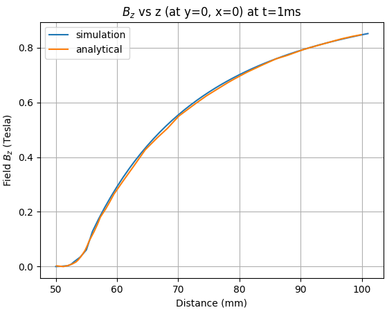
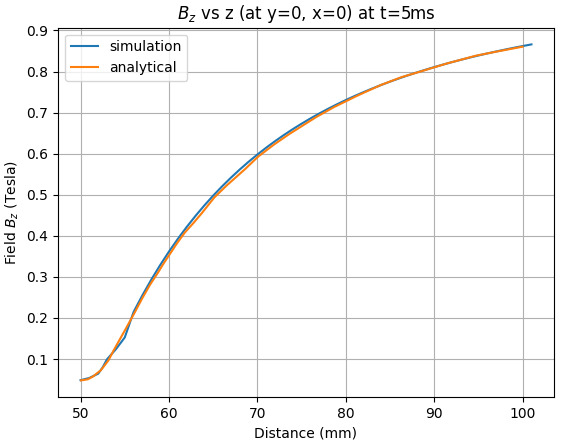
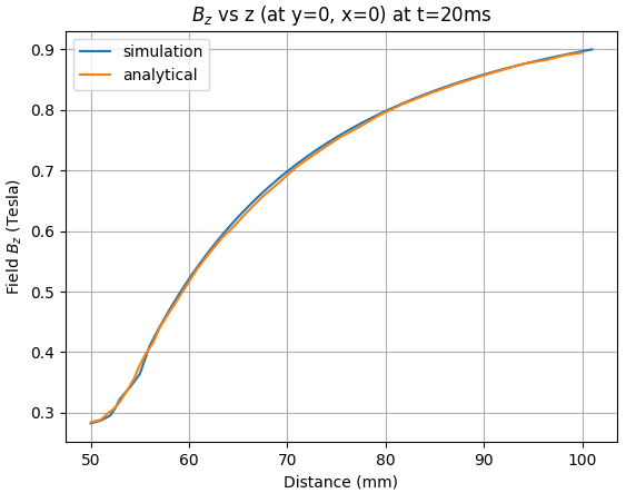
Table 5: z-Bfield for several z coordinates (at y = 0, x = 0) for 1 ms, 5 ms and 20 ms

Result	Target	LS-DYNA	Error (%)
z Field at t = 1 ms for z = 60 mm	0.29	0.29	0.93
z Field at t = 1 ms for z = 70 mm	0.53	0.55	5.00
z Field at t = 1 ms for z = 80 mm	0.70	0.70	0.44
z Field at t = 1 ms for z = 90 mm	0.78	0.79	0.95
z Field at t = 1 ms for z = 90 mm	0.78	0.79	0.95
z Field at t = 1 ms for z = 100 mm	0.85	0.85	0.05
z Field at t = 5 ms for z = 60 mm	0.36	0.36	1.52
z Field at t = 5 ms for z = 70 mm	0.58	0.60	3.47
z Field at t = 5 ms for z = 80 mm	0.73	0.73	0.34
z Field at t = 5 ms for z = 90 mm	0.81	0.81	0.12
z Field at t = 5 ms for z = 90 mm	0.81	0.81	0.12
z Field at t = 5 ms for z = 100 mm	0.86	0.86	0.17
z Field at t = 20 ms for z = 60 mm	0.52	0.52	0.11
z Field at t = 20 ms for z = 70 mm	0.69	0.70	0.77
z Field at t = 20 ms for z = 80 mm	0.80	0.80	0.22
z Field at t = 20 ms for z = 90 mm	0.86	0.86	0.13
z Field at t = 20 ms for z = 90 mm	0.86	0.86	0.13
z Field at t = 20 ms for z = 100 mm	0.89	0.90	0.27

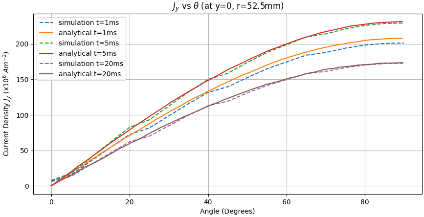
Table 6: Current Density for several angles (at y = 0, r = 52.5 mm) for 1 ms, 5 ms and 20 ms

Result	Target	LS-DYNA	Error (%)
Current Density at t = 1 mm ms for θ = 10 deg	37.59	34.69	7.71
Current Density at t = 1 ms for θ = 20 deg	72.34	72.48	0.19
Current Density at t = 1 ms for θ = 40 deg	131.74	131.67	0.05
Current Density at t = 1 ms for θ = 50 deg	157.62	152.41	3.31
Current Density at t = 1 ms for θ = 70 deg	194.33	187.75	3.38
Current Density at t = 1 ms for θ = 80 deg	205.14	198.19	3.39
Current Density at t = 1 ms for θ = 90 deg	207.80	201.07	3.24
Current Density at t = 5 ms for θ = 10 deg	38.52	39.54	2.66
Current Density at t = 5 ms for θ = 20 deg	80.21	82.60	2.98
Current Density at t = 5 ms for θ = 40 deg	149.65	149.80	0.11
Current Density at t = 5 ms for θ = 50 deg	174.38	173.86	0.30
Current Density at t = 5 ms for θ = 70 deg	216.96	213.95	1.39
Current Density at t = 5 ms for θ = 80 deg	227.74	225.85	0.83
Current Density at t = 5 ms for θ = 90 deg	231.10	229.13	0.85
Current Density at t = 20 ms for θ = 10 deg	28.62	29.79	4.09
Current Density at t = 20 ms for θ = 20 deg	58.83	62.23	5.78
Current Density at t = 20 ms for θ = 40 deg	112.37	112.80	0.39
Current Density at t = 20 ms for θ = 50 deg	133.04	130.89	1.62
Current Density at t = 20 ms for θ = 70 deg	163.78	161.13	1.62
Current Density at t = 20 ms for θ = 80 deg	170.67	170.13	0.32
Current Density at t = 20 ms for θ = 90 deg	173.50	172.61	0.51