VM-LSDYNA-EMAG-003

VM-LSDYNA-EMAG-003
Non-Linear Magnetostatic Problem

Overview

Reference:	Nakata, T. & Fujiwara, K. (1992) Summary of results for benchmark problem 13 (3-D nonlinear magnetostatic model). COMPEL-The International Journal for Computation and Mathematics in Electrical and Electronic Engineering, 11, 345-369.
Analysis Type(s):	Electromagnetism
Element Type(s):	Solid Elements ELFORM 1
Input Files:	Link to Input Files Download Page

Test Case

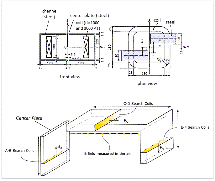
The TEAM 13 problem is a non-linear magnetostatic case where a coil excited by DC current is set between two steel channels not aligned with each other–with a steel plate inserted between the channels. This produces a three-dimensional magnetic field.

The number of turns in the coil is 1000, and the applied magnetomotive forces are either 1000 AT or 3000 AT, which is enough to reach steel saturation. These two forces are applied separately in two different simulations. The material properties are shown in the table below.

The goal is to determine the current density across the line shown in Figure 172, as well as at different sections for each steel plate, and compare it with the experimental results.

Figure 171: Problem sketch and dimensions (in mm, top figure) and location of the points/sections to measure the magnetic field

Figure 172: Problem setup

Material Properties	Loading
Young's modulus, steel = 2∙10¹¹ Pa Poisson's ratio, steel = 0.3 Density steel = 7000 kg/m³ Conductivity = 1.2∙10^-8 Ω∙m	Magnetomotive force_1 = 1000 AT Magnetomotive force_2 = 3000 AT

Material Properties

Young's modulus, steel = 2∙10¹¹ Pa

Poisson's ratio, steel = 0.3

Density steel = 7000 kg/m³

Conductivity = 1.2∙10^-8 Ω∙m

Magnetomotive force_1 = 1000 AT

Magnetomotive force_2 = 3000 AT

Analysis Assumptions and Modeling Notes

The results are time dependent by considering the conductivity of the plate (Eddy current diffusion). Since the problem itself is static, the latest time step is taken to verify the results.

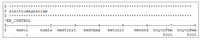
LS-DYNA *EM_CONTROL card is set to 1 to activate the Eddy Current solver.

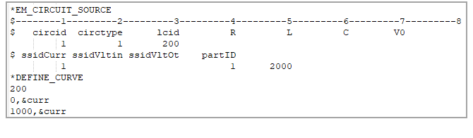
Magnetomotive forces are applied using *EM_CIRCUIT_SOURCE and defining the forces via *DEFINE_CURVE. The parameter &curr is the current, which corresponds to 1E6 (since, for 1000 coil turns, yields 1000 ampere-turn) for the 1000 AT case and 3E6 for the 3000 AT case.

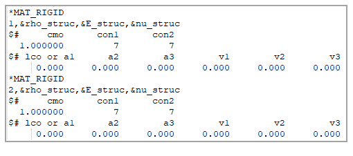
Rigid materials definition is applied to all components using MAT_RIGID.

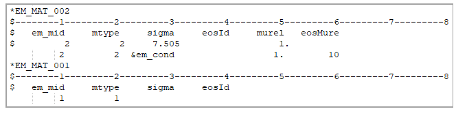
Electromagnetic properties are applied using EM_MAT_002 and EM_MAT_001.

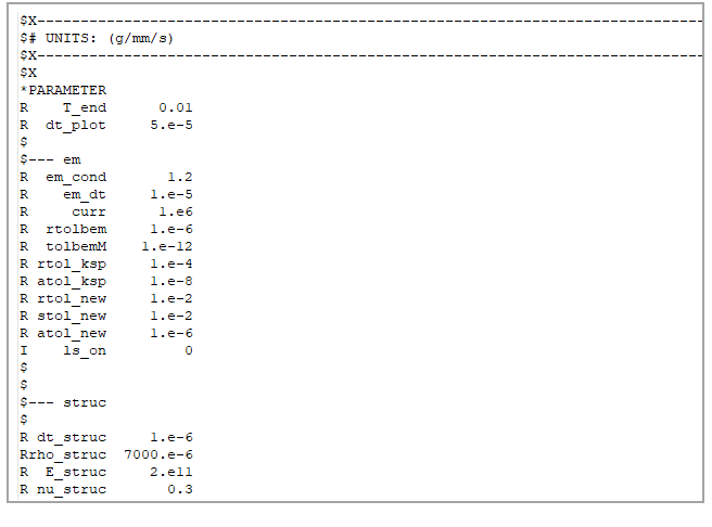
Finally, the properties are supplied parametrically and stored as parameters.

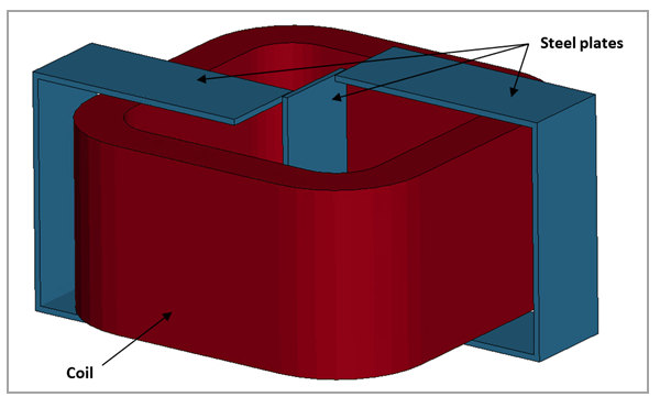
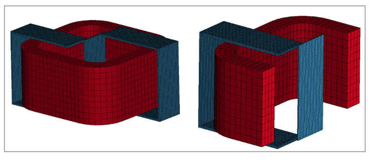
The mesh is formed by solid elements formulation 1, which is a constant stress solid element. Figure 173 shows the mesh as well as a cut section.

Figure 173: Mesh details

Results Comparison

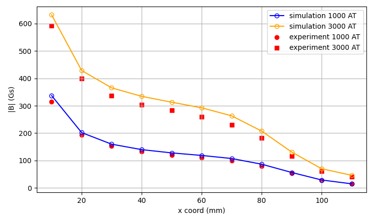
The experimental results are compared with LS-DYNA output. The magnetic field is obtained from two different files. Magnetic field for fixed points in the air is obtained from em_pointout.dat file. The results are compared against the experimental data for 1000 AT and 3000 AT in Figure 174.

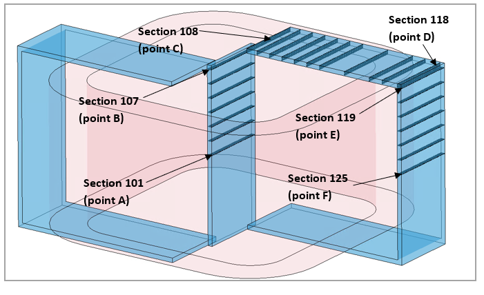
Figure 174: Simulation vs experiment results for 1000 and 3000 AT for points in air

The magnetic field in the steel channels is obtained from em_rogoCoil_XXX.dat files, and each file represents one of the sections (from 101 to 125) from which the magnetic filed is extracted. These sections are depicted in Figure 175. Results are shown in Figure 176.

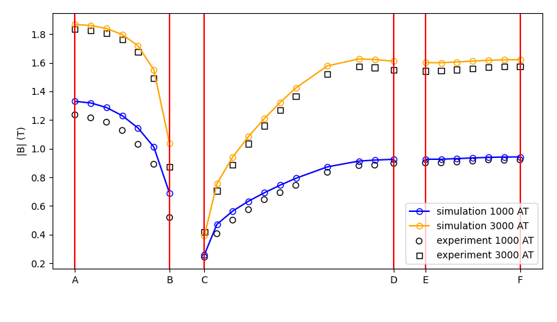
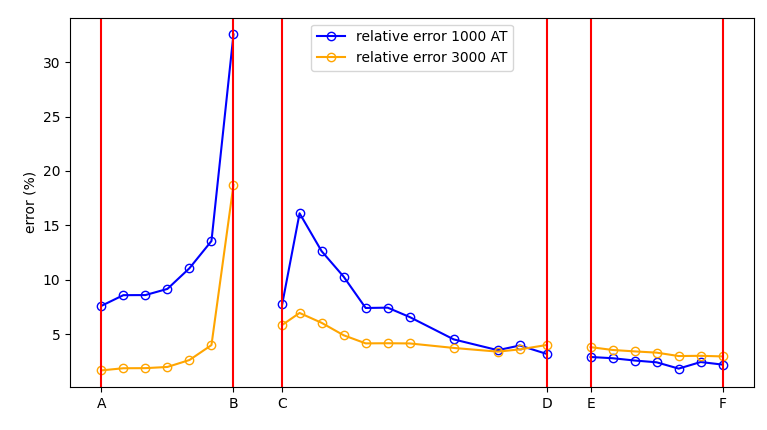
Figure 175: Sections at which magnetic field is extracted within the steel plates

Figure 176: Simulation vs experiment results for 1000 and 3000 AT for points in steel plates

The error between the experimental results and the simulation is presented in Table 7, Table 8, Table 9 and Table 10. The error curves are presented in Figure 177 and Figure 178. It is possible you will see that the results in the air are much closer to the experimental results for a lower value of magnetomotive force, while results in the steel sections show the opposite. There are several possible reasons for these discrepancies:

The experimental test setup could have introduced errors during the measurement.
Or the B-H curve of the steel may not be fully accurate and homogeneous, especially for high flux densities where an approximation is used. This can impact the final simulation results.
The steel plates are welded for the experiment, but this welding is not modelled in the simulation. This can also introduce discrepancies.
Finally, the coil modeling is an approximation that does not consider each wire of the coil. Each wire's magnetic field will interact with the others which also leads to discrepancies between experimental and simulation results.

Overall, the results are within a 15% error except for one point. For such a complex test, the simulation results represent a good approximation of reality.

Table 7: Magnetic field for in the air for 1000 AT

Result	Target	LS-DYNA	Error (%)
Bfield (T) at x = 10 mm	315.000	337.159	7.035
Bfield (T) at x = 20 mm	194.000	201.918	4.082
Bfield (T) at x = 30 mm	153.000	159.576	4.298
Bfield (T) at x = 40 mm	133.000	139.704	5.041
Bfield (T) at x = 50 mm	120.000	127.732	6.444
Bfield (T) at x = 60 mm	110.000	118.416	7.651
Bfield (T) at x = 70 mm	98.700	107.231	8.643
Bfield (T) at x = 80 mm	79.700	86.428	8.442
Bfield (T) at x = 90 mm	53.300	56.230	5.497
Bfield (T) at x = 100 mm	28.400	28.694	1.037
Bfield (T) at x = 110 mm	14.200	14.743	3.824

Table 8: Magnetic field for in the air for 3000 AT

Result	Target	LS-DYNA	Error (%)
Bfield (T) at x = 10 mm	593.00	632.28	6.62
Bfield (T) at x = 20 mm	400.00	428.89	7.22
Bfield (T) at x = 30 mm	336.00	365.37	8.74
Bfield (T) at x = 40 mm	304.00	334.45	10.02
Bfield (T) at x = 50 mm	283.00	312.94	10.58
Bfield (T) at x = 60 mm	260.00	292.41	12.47
Bfield (T) at x = 70 mm	231.00	263.18	13.93
Bfield (T) at x = 80 mm	182.00	207.31	13.90
Bfield (T) at x = 90 mm	116.00	130.95	12.89
Bfield (T) at x = 100 mm	61.00	69.78	14.39
Bfield (T) at x = 110 mm	40.60	45.91	13.08

Figure 177: Relative absolute error 1000 and 3000 AT between simulation and experiment for points in air

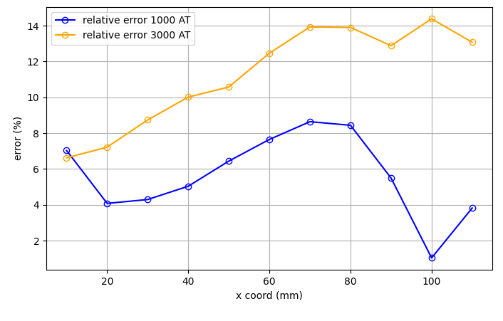
Table 9: Magnetic field for steel sections for 1000 AT

Result	Target	LS-DYNA	Error (%)
B-Field (T) for section 101	1.236	1.3299	7.60
B-Field (T) for section 102	1.215	1.3193	8.58
B-Field (T) for section 103	1.185	1.2868	8.59
B-Field (T) for section 104	1.127	1.2302	9.16
B-Field (T) for section 105	1.030	1.1439	11.06
B-Field (T) for section 106	0.891	1.0118	13.56
B-Field (T) for section 107	0.519	0.6879	32.54
B-Field (T) for section 108	0.242	0.2607	7.73
B-Field (T) for section 109	0.406	0.4714	16.11
B-Field (T) for section 110	0.501	0.5642	12.61
B-Field (T) for section 111	0.574	0.6330	10.28
B-Field (T) for section 112	0.644	0.6917	7.41
B-Field (T) for section 113	0.693	0.7445	7.43
B-Field (T) for section 114	0.744	0.7929	6.57
B-Field (T) for section 115	0.835	0.8727	4.51
B-Field (T) for section 116	0.882	0.9131	3.53
B-Field (T) for section 117	0.885	0.9200	3.95
B-Field (T) for section 118	0.897	0.9256	3.19
B-Field (T) for section 119	0.900	0.9261	2.90
B-Field (T) for section 120	0.901	0.9261	2.79
B-Field (T) for section 121	0.907	0.9304	2.58
B-Field (T) for section 122	0.913	0.9350	2.41
B-Field (T) for section 123	0.922	0.9389	1.83
B-Field (T) for section 124	0.919	0.9414	2.44
B-Field (T) for section 125	0.922	0.9423	2.20

Table 10: Magnetic field for steel sections for 3000 AT

Result	Target	LS-DYNA	Error (%)
B-Field (T) for section 101	1.836	1.8667	1.67
B-Field (T) for section 102	1.826	1.8602	1.87
B-Field (T) for section 103	1.805	1.8389	1.88
B-Field (T) for section 104	1.762	1.7971	1.99
B-Field (T) for section 105	1.674	1.7180	2.63
B-Field (T) for section 106	1.491	1.5506	4.00
B-Field (T) for section 107	0.872	1.0353	18.73
B-Field (T) for section 108	0.417	0.3926	5.85
B-Field (T) for section 109	0.706	0.7551	6.95
B-Field (T) for section 110	0.888	0.9417	6.05
B-Field (T) for section 111	1.034	1.0847	4.90
B-Field (T) for section 112	1.161	1.2092	4.15
B-Field (T) for section 113	1.269	1.3219	4.17
B-Field (T) for section 114	1.367	1.4237	4.15
B-Field (T) for section 115	1.521	1.5778	3.73
B-Field (T) for section 116	1.573	1.6264	3.39
B-Field (T) for section 117	1.566	1.6225	3.61
B-Field (T) for section 118	1.548	1.6100	4.01
B-Field (T) for section 119	1.542	1.6008	3.81
B-Field (T) for section 120	1.545	1.5998	3.55
B-Field (T) for section 121	1.552	1.6051	3.42
B-Field (T) for section 122	1.560	1.6116	3.31
B-Field (T) for section 123	1.570	1.6170	2.99
B-Field (T) for section 124	1.573	1.6204	3.01
B-Field (T) for section 125	1.575	1.6216	2.96

Figure 178: Relative absolute error for 1000 and 3000 AT between simulation and experiment for points in steel plates