


VM-LSDYNA-EMAG-001
VM-LSDYNA-EMAG-001
Conducting Ladder Below a Coil Carrying a Sinusoidal Current
Overview
| Reference: |
Turner, L R. (1988) Proceedings of the Vancouver team workshop at the University of British Columbia, USA, 13-14. Zheng, D. (1997). Three-dimensional eddy current analysis by the boundary element method. IEEE Transactions on Magnetics, 33, 1354-1357. Çaldichoury, I. & L’Eplattenier, P. Validation Process of the Electromagnetism (EM) solver in LS-DYNA v980: The TEAM problems. 2th International LS-DYNA Users Conference, Livermore, CA. |
| Analysis Type(s): | Electromagnetism |
| Element Type(s): | Solid elements ELFORM 1 |
| Input Files: | Link to Input Files Download Page |
Test Case
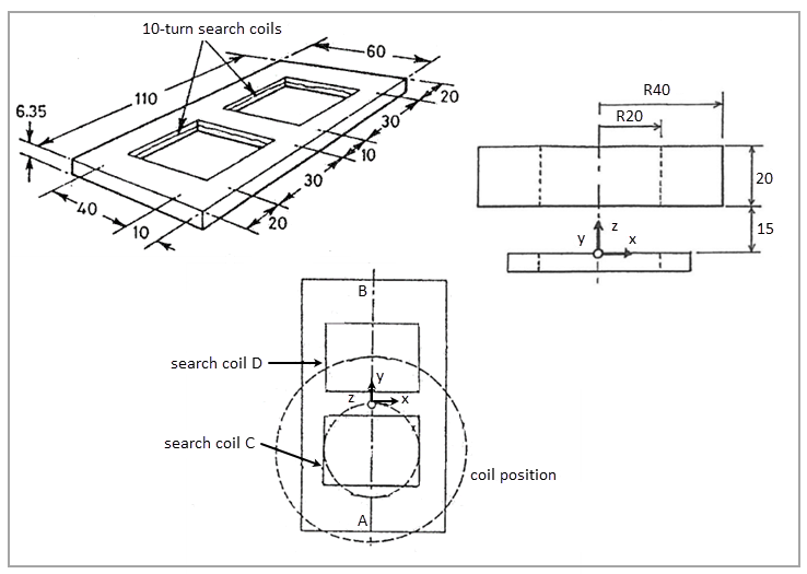
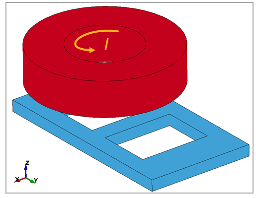
The TEAM 3 problem is a classic validation test and consists of a conducting ladder with two holes placed below a coil carrying a sinusoidal current. The coil is made of multiple turns strongly stranded together, so the current in the coil is considered uniform (no eddy currents) while the ladder's induced current diffuses through its thickness. The coil is located directly above one of the holes. The problem sketch, with dimensions, is shown in Figure 164.
The coil sees a 1260 ampere-turn current and oscillates at a frequency of 50 Hz while the ladder has a conductivity of 32.78E+06 Ω-1m-1.
The objective of the test is to study the behavior of the magnetic field along a line that goes from (x = 0, y = -55, z = 0.5) mm to (x = 0, y = 55, z = 0.5) mm. The coordinate system is shown in the problem sketch. The results are then compared to the experimental results in the reference.
| Material Properties | Loading |
|---|---|
| Conductivity = 32.78∙106 Ω-1 m-1 | I = 1260 A |
Analysis Assumptions and Modeling Notes
>LS-DYNA *EM_CONTROL card is set to 1 to activate the Eddy Current solver. The current is applied using *EM_CIRCUIT_SOURCE card.
In addition, the Biot-Savart approach is used to compute the results.
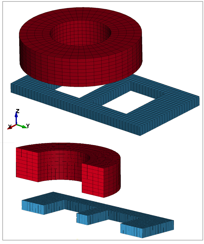
The mesh is formed by solid elements formulation 1 which is a constant stress solid element. The ladder mesh contains eight elements across its thickness for better accuracy.
Results Comparison
The experimental results are compared with LS-DYNA output. Simulation results are extracted from the em_pointout.dat file.
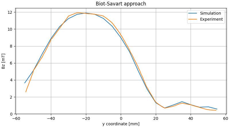
The error between the experimental results and the simulation is presented in the table below. It is possible to see that only two points have a higher discrepancy compared to the experiment. These discrepancies can be due to the disregard of eddy currents during the simulation, since the coils contain insulation layers that make the current density non-homogeneous. Nevertheless, there is a good agreement between simulation and experimental results.
Table 3: z-Bfield for several y coordinates (at x = 0, z = 0.5)
| Result | Target | LS-DYNA | Error (%) |
| z-Bfield [mT] at y = -50 mm | 5.13 | 5.16 | 0.73 |
| z-Bfield [mT] at y = -40 mm | 8.89 | 8.80 | 1.03 |
| z-Bfield [mT] at y = -30 mm | 11.23 | 11.55 | 2.71 |
| z-Bfield [mT] at y = -20 mm | 11.90 | 11.85 | 0.37 |
| z-Bfield [mT] at y = -10 mm | 11.26 | 11.55 | 2.49 |
| z-Bfield [mT] at y = 0 mm | 8.99 | 9.27 | 3.09 |
| z-Bfield [mT] at y = 10 mm | 5.04 | 5.40 | 6.60 |
| z-Bfield [mT] at y = 20 mm | 1.31 | 1.38 | 5.35 |
| z-Bfield [mT] at y = 30 mm | 1.05 | 0.91 | 15.53 |
| z-Bfield [mT] at y = 40 mm | 1.08 | 1.09 | 0.86 |
| z-Bfield [mT] at y = 50 mm | 0.83 | 0.50 | 66.47 |