VM-LSDYNA-EMAG-007
VM-LSDYNA-EMAG-007
2D Axisymmetric Inductive Heating
Overview
| Reference: |
Jankowski T., Pawley, N., Gonzales, L., Ross, C., & Jurney, J. (2016). Approximate analytical solution for induction heating of solid cylinders. Annual Mathematical Modelling, 4(40), 2770-2782. https://www.dynaexamples.com/em/eddycurr/2dindheat |
| Analysis Type(s): | Electromagnetism |
| Element Type(s): | Solid Elements ELFORM 1 |
| Input Files: | Link to Input Files Download Page |
Test Case
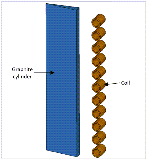
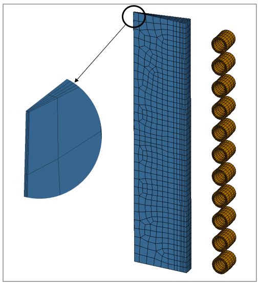
In this test case, a heated coil is wrapped around a cylinder. The coil carries a sinusoidal current and has 11 turns. Since the model is symmetric, only a portion of it is modelled to reduce computation time as shown in Figure 196. Model dimensions are given in Table 13 and Figure 195.The material properties are shown in Table 14.
The test case replicates only the first experiment in the reference. The goal is to determine the temperature at the bottom center of the cylinder where the temperature sensor is located in the experiment.
Table 13: Model dimensions
| T∞ 293.15 K | I(RMS) %I* 1063 A | ||||||||
|
|
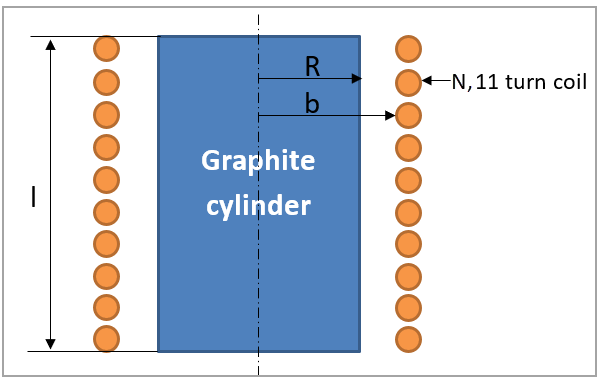
Table 14: Material properties of POCO grapite
| Material Properties of POCO grapite | ||||
| T(K) | σ(1/Ωm) | c(J/kg K) | k(W/m K) | ρ(kg/m3) |
| 293.15 | 75,250 | 721 | 120 | 1720 |
| 393.15 | 86,417 | 1026 | 108 | 1720 |
| 493.15 | 96,585 | 1269 | 95 | 1720 |
| 593.15 | 105,001 | 1424 | 88 | 1720 |
| 693.15 | 111,244 | 1549 | 80 | 1720 |
| 793.15 | 115,292 | 1645 | 75 | 1720 |
| 893.15 | 117,437 | 1712 | 70 | 1720 |
| 993.15 | 118,124 | 1763 | 66 | 1720 |
| 1093.15 | 117,807 | 1809 | 62 | 1720 |
| 1193.15 | 116,860 | 1855 | 60 | 1720 |
| 1293.15 | 115,549 | 1892 | 57 | 1720 |
| 1393.15 | 114,035 | 1926 | 56 | 1720 |
| 1493.15 | 112,396 | 1959 | 55 | 1720 |
Analysis Assumptions and Modeling Notes
When considering the conductivity of the plate (eddy current diffusion), the results are time dependent. The latest time step is taken to verify the results since the problem itself is static.
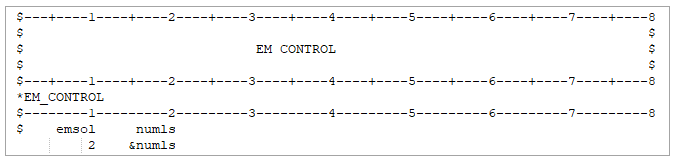
LS-DYNA *EM_CONTROL card is set to 1 to activate the eddy current solver:
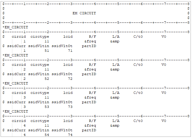
Intensity applied to the coils is given individually for each coil using *EM_CIRCUIT_SOURCE.
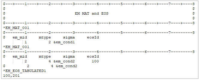
Electromagnetic properties are given using EM_MAT_002 and EM_MAT_001.
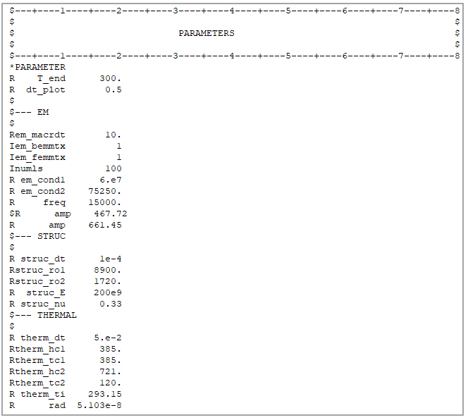
Finally, the properties are given parametrically and stored as parameters.
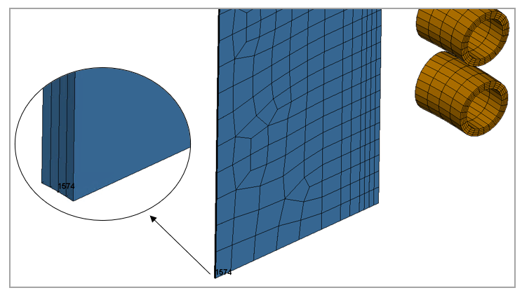
The mesh is formed by solid elements formulation 1, which is a constant stress solid element. There are four elements across the cylinder thickness. Figure 197 shows the mesh as well as a mesh detail.
Results Comparison
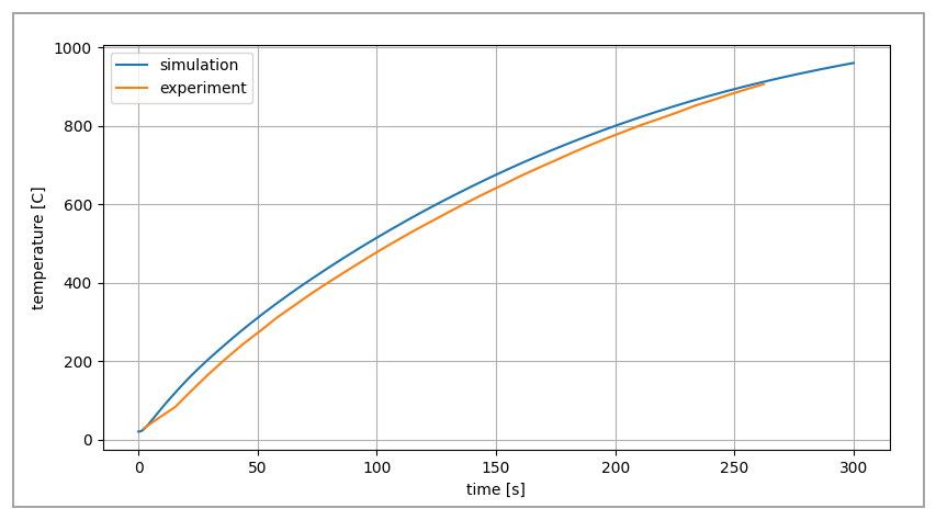
The experimental results are compared with LS-DYNA output in Figure 198. As you can see, the difference between both curves is reduced as the simulation time increases and gets very close at the end. The initial discrepancy is related to how the experiment is configured which causes the cylinder to heat up very quickly. This results in a significant temperature gradient between the heated zone and the bottom of the load, causing the discrepancies. As a result, the very first 50 seconds are disregarded when calculating the error.
The temperature is obtained from the d3plot files, specifically from node 1574 at the bottom of the cylinder where the temperature sensor is located in the experiment is (see Figure 199).
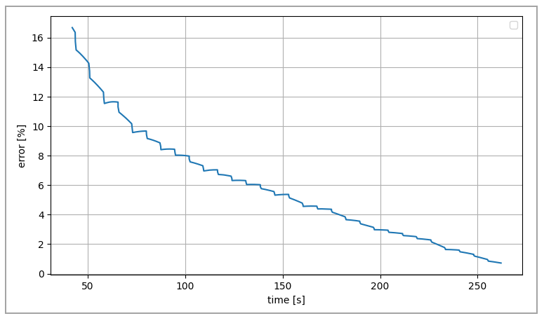
The error between the experimental results and the simulation is presented in the table below. The error curve is presented in Figure 200: Relative error between simulation and experiment. As you can see, the error decreases as the simulation progresses, leading to a very close result as the final temperature is reached.
| Result | Target | LSDYNA App | Error (%) |
| Temperature at t = 42 sec | 232.45 | 271.24 | 16.69 |
| Temperature at t = 56 sec | 300.19 | 338.07 | 12.62 |
| Temperature at t = 70 sec | 360.84 | 398.70 | 10.49 |
| Temperature at t = 84 sec | 417.16 | 454.82 | 9.03 |
| Temperature at t = 98 sec | 469.65 | 507.35 | 8.03 |
| Temperature at t = 112 sec | 520.12 | 556.61 | 7.02 |
| Temperature at t = 126 sec | 566.88 | 602.74 | 6.33 |
| Temperature at t = 140 sec | 610.89 | 645.95 | 5.74 |
| Temperature at t = 154 sec | 653.00 | 686.37 | 5.11 |
| Temperature at t = 168 sec | 693.54 | 723.97 | 4.39 |
| Temperature at t = 182.3 sec | 732.05 | 759.46 | 3.74 |
| Temperature at t = 196.5 sec | 768.02 | 792.16 | 3.14 |
| Temperature at t = 210.5 sec | 800.05 | 821.92 | 2.73 |
| Temperature at t = 224.5 sec | 830.23 | 849.40 | 2.31 |
| Temperature at t = 238.5 sec | 860.72 | 874.62 | 1.61 |