VM-LSDYNA-EMAG-008
VM-LSDYNA-EMAG-008
Magnetostatic Force Calculation (TEAM 20)
Overview
| Reference: | Takahashi, N., Nakata, T. & Morishige, H. (1995) Summary of results for problem 20 (3‐D static force problem). COMPEL-The International Journal for Computation and Mathematics in Electrical and Electronic Engineering, 14 (2/3), 57-75. |
| Analysis Type(s): | Electromagnetism |
| Element Type(s): | Solid Elements ELFORM 1 |
| Input Files: | Link to Input Files Download Page |
Test Case
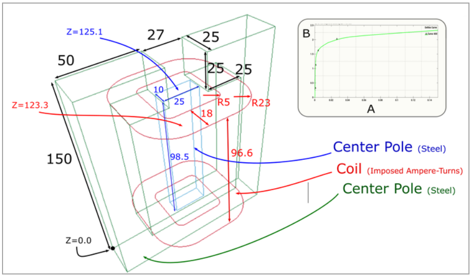
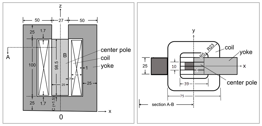
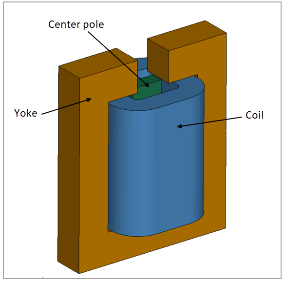
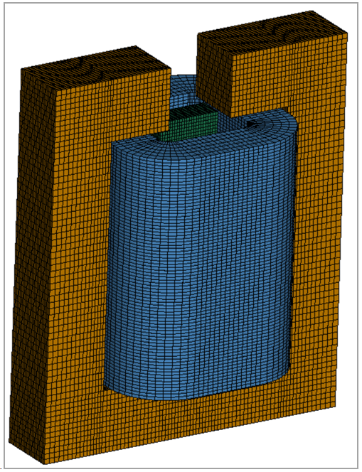
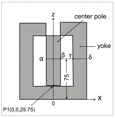
The TEAM 20 problem is a non-linear, magnetostatic, 3D model designed to verify magnetostatic force calculations. The center pole and yoke are made of steel. The coil is a source circuit with imposed ampere-turns. The model allows you to investigate surface magnetic force calculations obtained by the LS-DYNA monolithic solver in magnetostatic cases under different current excitations.
The goal is to determine flux densities at specific surface points within the model as well as the magnetostatic force for different values of ampere-turns. Results are then compared to experimental results in the reference.
Analysis Assumptions and Modeling Notes
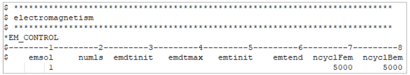
LS-DYNA *EM_CONTROL card is set to 1 to activate the Eddy Current solver.
The ampere-turns are specified using a load case within *EM_CIRCUIT_SOURCE. The &curr corresponds to the different values of current intensity for each timestep of the simulation. This way, it is possible to analyze different current intensities within the same simulation—that is, one simulation handles several static problems.
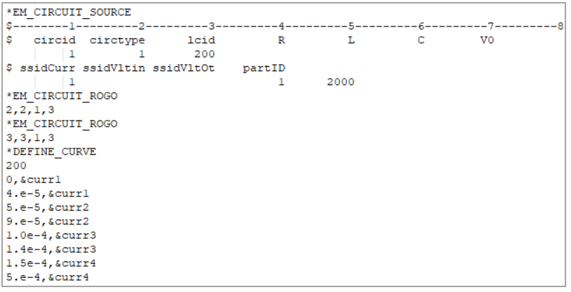
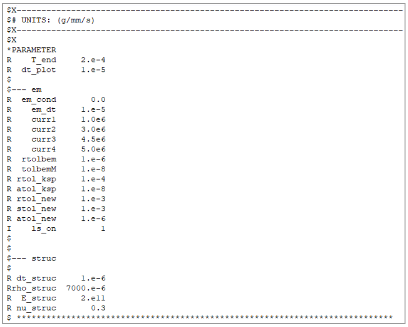
The current values as well as others are parametrized.
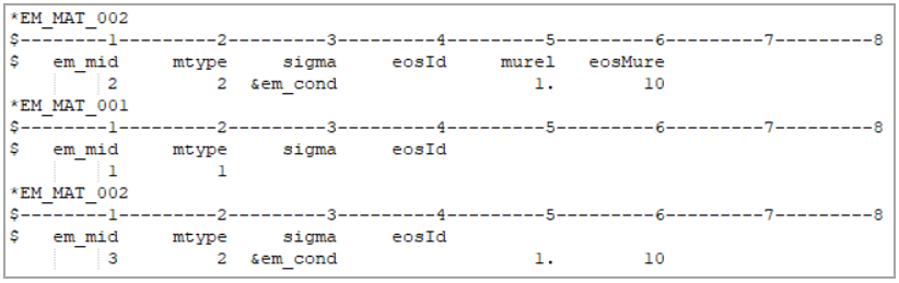
Finally, electromagnetic properties are given using EM_MAT_002 and EM_MAT_001.
The mesh is formed by solid elements formulation 1, which is a constant stress solid element.
Results Comparison
The following results are extracted and compared against the experimental results:
Bz flux densities at point (0,0,25.75)
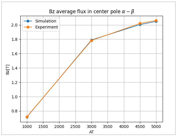
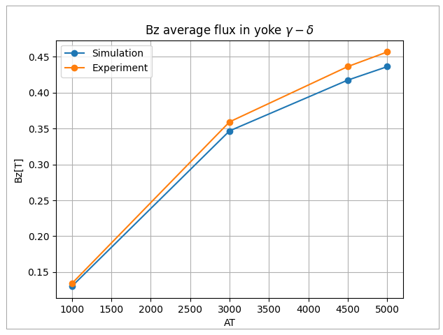
Bz average flux densities along the lines α-β (center pole) and ϒ-δ (yoke)
Fz electromagnetic force
The point of interest as well as α-β (center pole) and ϒ-δ (yoke) lines are shown in Figure 205.
Point information is retrieved from em_pointout.dat file. Information for α-β as well as ϒ-δ is retrieved from em_rogoCoil_002.dat and em_rogoCoil_003.dat, respectively. Information provided in em_rogoCoil files are per area, which means that results must be divided by the cross area before comparing them to the experimental results.
Reference results are compared to the LS-DYNA output in Figure 206, Figure 207, Figure 208, and Figure 209. As you can see, there is a good correlation between them.
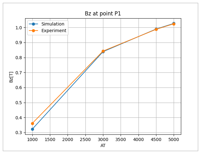
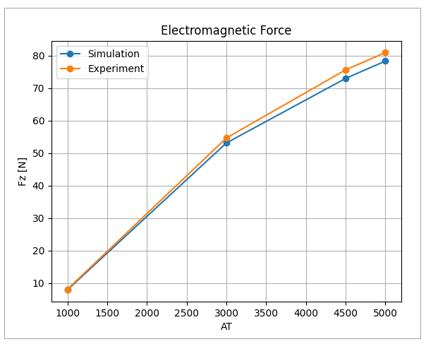
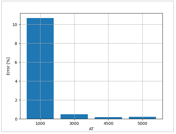
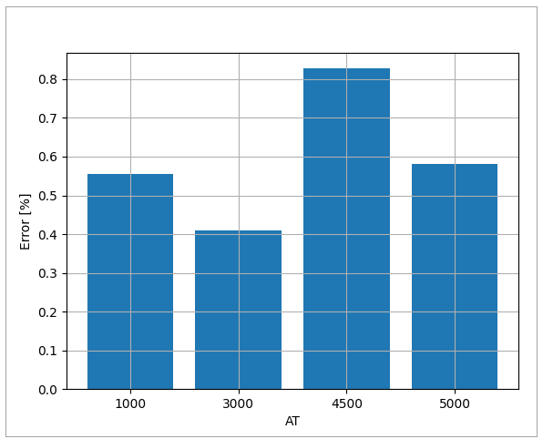
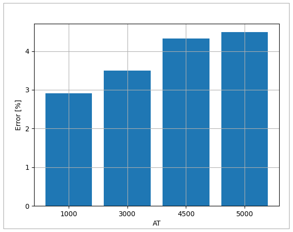
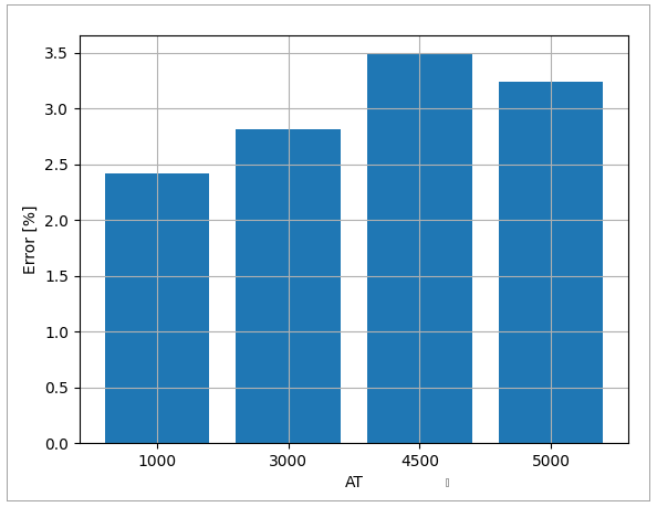
The error between the experimental results and the simulation at different ampere-turn values is presented in the bar charts below: Figure 210, Figure 211, Figure 212, and Figure 213. Errors remain below 4.5% except for point (0,0,25.75) at 1000 AT in Figure 210. This discrepancy is likely due to the difficulty of measuring this very narrow location during the experiment.