VM-LSDYNA-EMAG-006

VM-LSDYNA-EMAG-006
Voltage Driven Coil

Overview

Reference:	Leonard, P. J. & Rodger, D. (1988). Voltage forced coils for 3D finite-element electromagnetic models. IEEE Transactions on Magnetics, 24(6).
Analysis Type(s):	Electromagnetism
Element Type(s):	Solid Elements
Input Files:	Link to Input Files Download Page

Test Case

In this test case, a stranded coil is voltage driven rather than having an imposed current. The current is deduced from the specified voltage, the number of windings, and the coil's total resistance. Properties for both coil and plates are given in the table below. The goal of the test is to predict the coil's current under the influence of the conducting plates and compare it with the experimental results.

Coil Properties

Plate Properties

Inner radius = 0.087 m

Outer radius = 0.116 m

Height = 0.028 m

Resistance = 12.4 Ω

Voltage = 20 volts/step

Length = 0.24 m

Width = 0.24 m

Thickness = 0.0127 m

Conductivity = 3.28∙10⁷ m^-1

Separation = 0.03435 m

Figure 190: Problem sketch: Coil between two aluminum plates

Analysis Assumptions and Modeling Notes

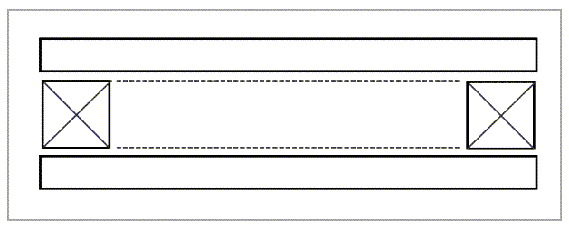
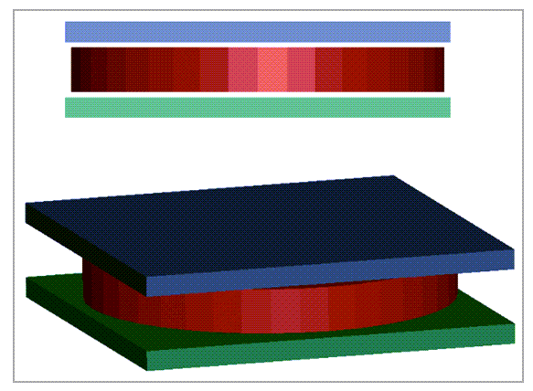
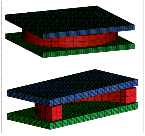
The LS-DYNA model is shown below. The plates are depicted as blue and green. The coil is red.

Figure 191: LS-DYNA Model

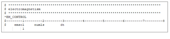
LS-DYNA *EM_CONTROL card is set to 1 to activate the Eddy Current solver.

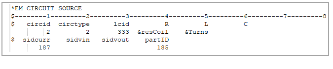
Coil properties, such as the number of turns, are given via *EM_CIRCUIT_SOURCE card.

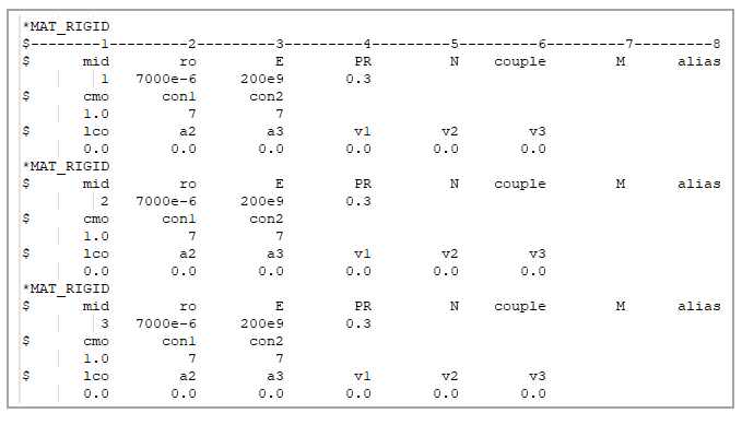
Rigid materials definition is used via MAT_RIGID for all the components.

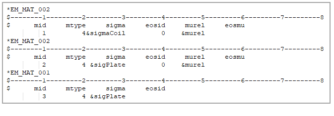
Electromagnetic properties are given to the plates and coil using EM_MAT_002 and EM_MAT_001.

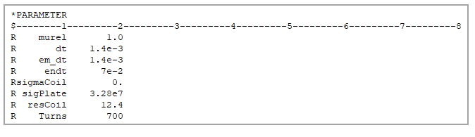
Finally, some properties are given parametrically and stored as parameters.

The mesh is formed by solid elements with Formulation 1, which is a constant stress solid element. Four elements are generated across the plate’s thickness for better accuracy. Two Elements are used for the coil.

Figure 192: Overall mesh and cut section

Results Comparison

Experimental and simulation results are compared in Figure 193. Simulation results are extracted from output file em_circuitSource_002.dat.

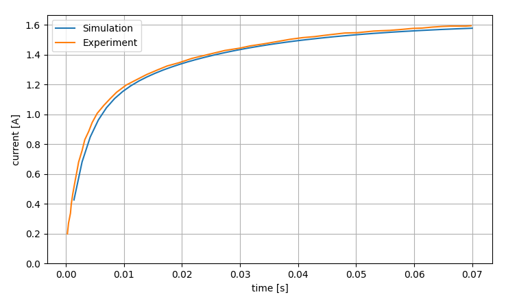
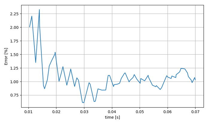
Figure 193: Simulation vs experiment plot

In the table below, the error is given for several time increments. The discrepancy is below 3% which is a good correlation between the solver and the experiment. Figure 194 shows the relative error across the simulation.

Result	Target	LS-DYNA	Error (%)
current [A] at t = 0.0104 s	1.172	1.196	2.007
current [A] at t = 0.019533 s	1.326	1.347	1.509
current [A] at t = 0.028 s	1.419	1.433	1.023
current [A] at t = 0.0378 s	1.483	1.496	0.843
current [A] at t = 0.0462 s	1.520	1.536	0.993
current [A] at t = 0.0546 s	1.547	1.561	0.932
current [A] at t = 0.063 s	1.566	1.583	1.072
current [A] at t = 0.0698 s	1.577	1.594	1.073

Figure 194: Relative error for several timesteps