


VM-LSDYNA-EMAG-005
VM-LSDYNA-EMAG-005
Lenz's Law: Magnet Through a Copper Pipe
Overview
| Reference: | Levin, Y., da Silveira, F. & Rizzato, F. (2006). Electromagnetic braking: a simple quantitative model. American Journal of Physics, 74(815). https://doi.org/10.1119/1.2203645 |
| Analysis Type(s): | Electromagnetism |
| Element Type(s): | Solid Elements |
| Input Files: | Link to Input Files Download Page |
Test Case
This test case, which was developed to demonstrate the Lenz Law, consists of a long metal pipe (in this case, made of copper) placed vertically along the Z axis. A magnet is placed at its top aperture. According to Lenz, once the magnet is released, its travel time through the pipe will be longer than a non-magnetic object.
The test compares the terminal velocity, which is the average velocity of the magnet while travelling through the pipe, of the analytical and the simulation solution. The only acting external force is gravity. The following geometrical and material properties are considered.
| Material Properties | Geometric Properties | Loading |
|---|---|---|
|
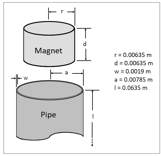
Copper conductivity = 1.75∙106-8 Ω m Magnet magnetization = 312739 A/m Magnet mass = 0.0029914 kg |
Pipe internal radius = 0.00785 m Magnet radius = 0.00635 m Magnet thickness = 0.00635 m Pipe thickness = 0.0019 m Pipe length = 0.0635 m |
g = 9.81 m/s2 |
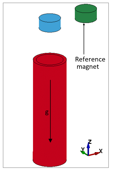
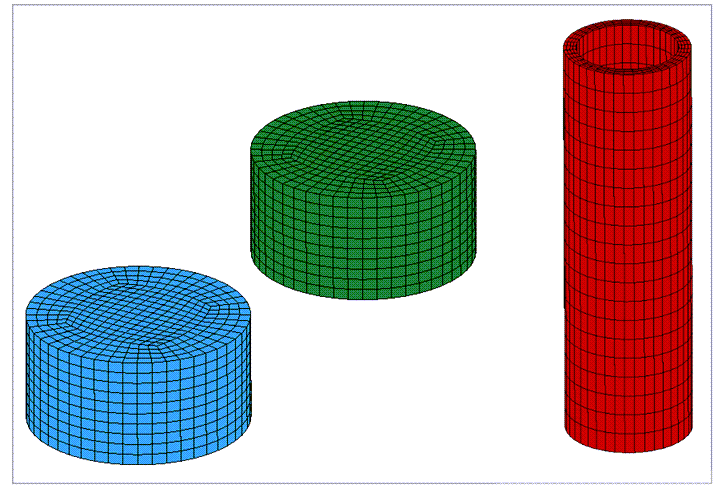
The LS-DYNA model is shown in Figure 186. The copper pipe (red) and the magnet placed on top of it (blue) are depicted. A reference magnet (green) is also modelled and serves as a reference to compare with the free fall time of a magnet that doesn't pass through a pipe.
Analysis Assumptions and Modeling Notes
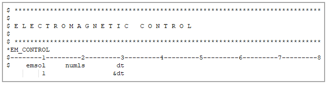
LS-DYNA *EM_CONTROL card is set to 1 to activate the Eddy Current solver.
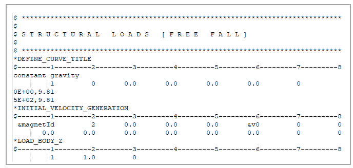
Gravity is applied only to the Z axis and to the magnets. No further boundary conditions are used.
Rigid materials definition is used via MAT_RIGID for all the components.
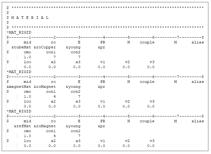
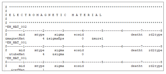
Electromagnetic properties are given to the magnets and the pipe using EM_MAT_002 and EM_MAT_001 respectively.
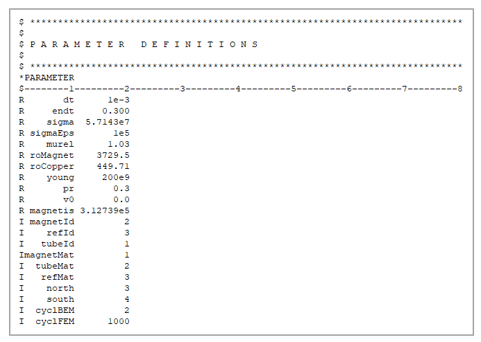
Finally, the properties are given parametrically and stored as parameters.
The mesh is formed by solid elements with formulation 1, which is a constant stress solid element. Four elements are generated across the pipe's thickness for better accuracy.
Results Comparison
The theoretical results are compared with the simulation results. The terminal velocity is
calculated theoretically and compared against the velocity  , where l is the length of the copper pipe and t is the time is takes for the
magnet to pass through the pipe. From the reference, the terminal velocity can be calculated
as:
, where l is the length of the copper pipe and t is the time is takes for the
magnet to pass through the pipe. From the reference, the terminal velocity can be calculated
as:
 | (28) |
Where a, w, d, and r, are geometrical properties found in Figure 185, ρ is the electrical
conductivity of the copper pipe, μ0 is the permeability of vacuum
(12.57e-7 H/m), M is the magnetization, m is the mass of the magnet, g is the
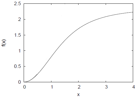
gravity acceleration and  is a scaling function defined as:
 | (29) |
This function can be plotted for small x as shown in Figure 188.
Considering the following parameters:
m = 0.0029914 kg
g = 9.81 m/s2
ρ = 1.75∙10-8 Ωm
a = 0.00785 m
μ0 = 12.57∙10-7 H/m
r = 0.00635 m
M = 312739 A/m
w = 0.0019 m
f(d/a) ≅ 0.5
The terminal velocity results in: 
To determine the velocity in the simulation, the time at which the magnet enter the pipe is noted, as well as the time at which the magnet starts leaving the pipe. From Figure 189, both times can be extracted. These are 0.06399 seconds and 0.25699 seconds, respectively.
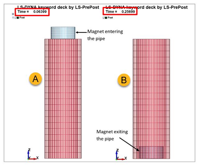
With initial and final time as well as the pipe length, the terminal velocity for the simulation is:
 | (30) |
The error between the theorical results and the simulation is presented in Table 12. The discrepancy is below a 3% which shows the good correlation between the solver and the simplified solution of Lenz law.
Table 12: Comparison between target (theorical value) and simulation results
| Result | Target | LS-DYNA | Error (%) |
| Terminal velocity [m/s] | 0.338 | 0.329 | 2.544 |