VM-LSDYNA-EMAG-004
VM-LSDYNA-EMAG-004
Axisymmetric Electrodynamic Levitation Problem
Overview
| Reference: |
Karl, H. & Fetzer, J. (1988). Description of team workshop problem 28: An electrodynamic levitation device. Institut fur Theorie der Elektrotechnik, Universitat Stuttgart, Pfa enwaldring 47, 70550, Stuttgart, Germany. Caldichoury, I. & L’Eplattenier, P. Validation Process of the Electromagnetism (EM) solver in LS-DYNA v980: The TEAM problems. 12th International LS-DYNA Users Conference, Livermore, CA. |
| Analysis Type(s): | Electromagnetism |
| Element Type(s): | Solid Elements ELFORM 1 |
| Input Files: | Link to Input Files Download Page |
Test Case
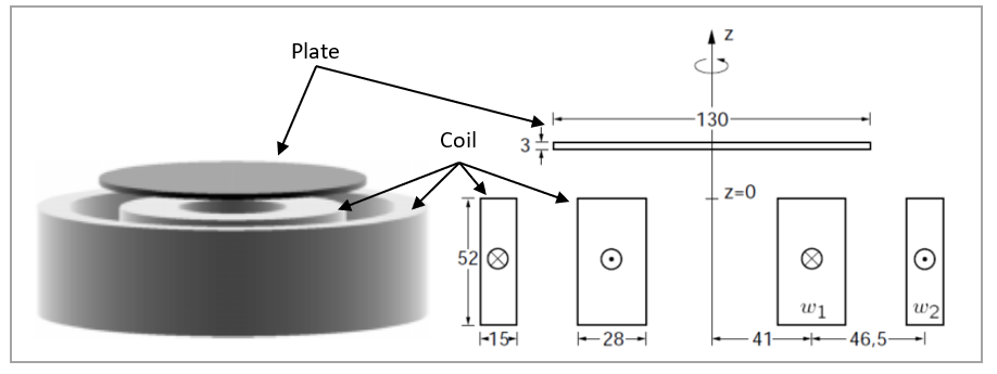
The TEAM 28 problem consists of an electrodynamic levitation device with a conducting plate which levitates over two exciting coils. The two coils have 20 turns. The interior coil has a current amplitude of 960 A, whereas the second one has 560 A. Both have a current frequency of 50 Hz. The plate has a conductivity of 34∙106 Ω-1m-1 and a density of 2687 kg∙m-3. The dimensions are shown in Figure 179.
The goal is to determine the axial displacement of the plate in time and compare it to the experimental solution.
| Material Properties | Loading |
|---|---|
|
Conductivity= 34∙106Ω-1m-1 ρ = 2687 kg∙m-3 |
Iint coil = 960 A Iext coil = 560 A |
Analysis Assumptions and Modeling Notes
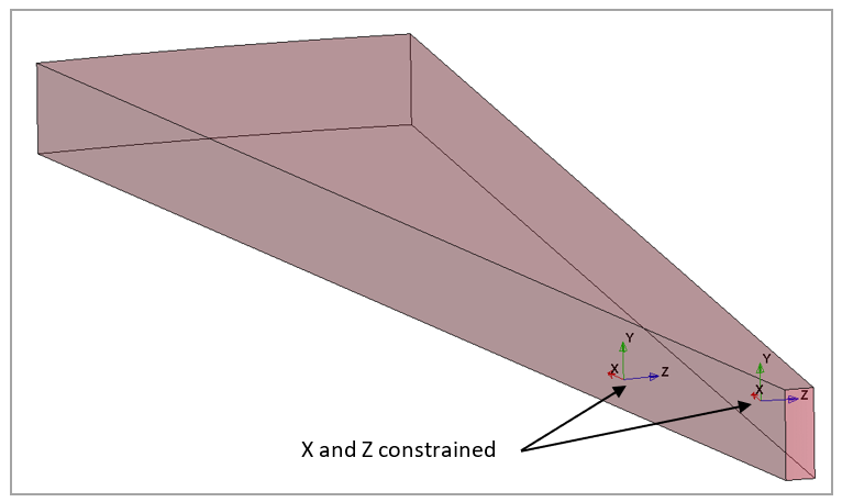
The test is a coupled problem between the solid mechanics solver and the electromagnetic solver. The LS-DYNA *EM_CONTROL card is set to 1 to activate the Eddy Current solver. Boundary conditions are applied to the plate to represent the axisymmetric problem. This constrains the lateral movement and releases the axial one. The correct constraint directions are obtained by means of secondary coordinate systems which ensure the axes are aligned with the lateral faces of the plate.
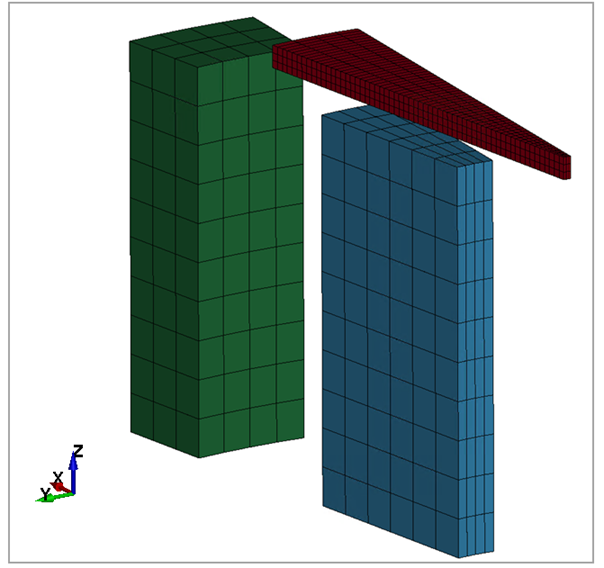
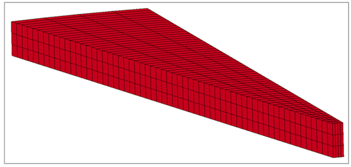
The mesh is formed by solid elements formulation 1, which is a constant stress solid element. The mesh of the plate contains three elements through the thickness for better accuracy.
Results Comparison
The experimental results are compared with the LS-DYNA output. The displacement of the plate's upper face is plotted in Figure 183.
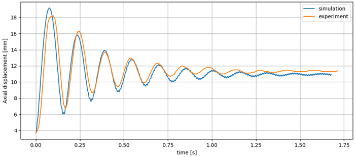
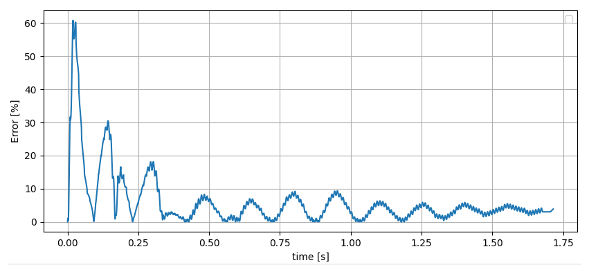
The error between the experimental results and the simulation is presented in Table 11 for selected points. The error curve is presented in Figure 184. Overall, the simulation results correlate nicely with the experimental solutions.
As seen in Figure 184, there is a higher discrepancy in the first half of the period. For numerical purposes, the cross section of the coils is approximated by a rectangle and carry a homogeneous azimuthal current density. The coils are made of copper wire which contain insulation layers, so the real current density is neither strictly homogeneous nor sharply bounded by a rectangle. These effects may influence the plate during its initial lift-off phase, which explains the bigger discrepancy in the maximum levitation height during the first half period.
Table 11: Axial displacement error for several time steps
| Result | Target | LSDYNA | Error (%) |
| z-disp [mm] (t = 0 s) | 3.70 | 3.70 | 0.00 |
| z-disp [mm] ( t = 0.09 s) | 18.36 | 18.12 | 1.33 |
| z-disp [mm] ( t = 0.27 s) | 12.19 | 14.09 | 13.46 |
| z-disp [mm] ( t = 0.36 s) | 12.42 | 12.13 | 2.42 |
| z-disp [mm] ( t = 0.55 s) | 12.77 | 12.90 | 1.02 |
| z-disp [mm] ( t = 0.64 s) | 9.82 | 10.39 | 5.51 |
| z-disp [mm] ( t = 0.82 s) | 11.09 | 11.81 | 6.05 |
| z-disp [mm] ( t = 0.91 s) | 10.65 | 11.00 | 3.17 |
| z-disp [mm] ( t = 1 s) | 11.40 | 11.72 | 2.70 |
| z-disp [mm] ( t = 1.18 s) | 11.11 | 11.18 | 0.63 |
| z-disp [mm] ( t = 1.27 s) | 10.84 | 11.40 | 4.95 |
| z-disp [mm] ( t = 1.36 s) | 10.80 | 11.20 | 3.54 |
| z-disp [mm] ( t = 1.45 s) | 10.97 | 11.40 | 3.73 |
| z-disp [mm] ( t = 1.54 s) | 10.82 | 11.38 | 4.95 |
| z-disp [mm] ( t = 1.64 s) | 11.00 | 11.30 | 2.69 |