13.4. Pressure Drop Calculations for Grilles

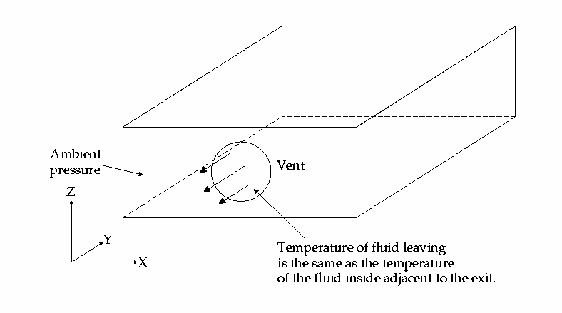
Ansys Icepak computes the speed, direction, and temperature of the fluid exiting the cabinet through a grille (see Figure 13.2: Outlet Grille Conditions (Vents)). The calculations are based on the assumption that the external pressure is static. If you do not specify a value for the external pressure, Ansys Icepak uses the ambient pressure specified under Ambient conditions in the Basic parameters panel (see Ambient Values).

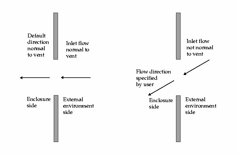
Figure 13.2: Outlet Grille Conditions (Vents)

Fluid entering the cabinet through a grille is drawn in from the external environment. By default, the external fluid is at the ambient temperature specified under Ambient conditions in the Basic parameters panel (see Ambient Values), and the flow enters the cabinet in a direction computed by Ansys Icepak. However, you can impose a flow direction, as shown in Figure 13.3: Grille Flow Direction (Vents). You can also specify a temperature for the fluid entering the grille.

Figure 13.3: Grille Flow Direction (Vents)

To account for pressure losses due to the presence of mesh screens or angled slats on the grille, you must specify a loss coefficient or select a grille type. See [ 11 ] for a compilation of loss coefficients applicable to most situations encountered in electronic enclosures.

Ansys Icepak can calculate loss coefficients for different types of grilles based on the free area ratio of the grille. The following grille types are available in Ansys Icepak:

a perforated thin vent, with a loss coefficient of
(13–1)
where A is the free area ratio.
a circular metal wire screen, with a loss coefficient of
(13–2)
where A is the free area ratio.
a two-plane screen with cylindrical bars, with a loss coefficient of
(13–3)
where A is the free area ratio.

Note: Setting the ambient temperature and flow direction has no effect on the calculations if fluid flows out of the cabinet through the vent.

Alternatively, Ansys Icepak can calculate the pressure drop resulting from a resistance either by the approach-velocity method or by the device-velocity method.

The approach-velocity method relates the pressure drop to the fluid velocity:

(13–4)

where l_c is the user-specified loss coefficient, ρ is the fluid density, and v_app is the approach velocity. The approach velocity is the calculated velocity at the plane of the grille. The velocity dependence can be linear (n = 1), quadratic (n = 2), or a combination of linear and quadratic.

The device-velocity method relates the pressure drop induced by the grille to the fluid velocity:

(13–5)

where v_dev is the device velocity. The velocity dependence can be linear (n = 1), quadratic (n = 2), or a combination of linear and quadratic.

The difference between the approach-velocity and device-velocity methods is in the velocity used to compute the pressure drop. The device velocity is related to the approach velocity by

(13–6)

where A is the free area ratio. The free area ratio is the ratio of the area through which the fluid can flow unobstructed to the total planar area of the obstruction.

Note: The loss coefficient used in the equation for the device velocity is not the same as the loss coefficient used in the equation for the approach velocity.

The loss coefficients in Equation 13–4 and Equation 13–5 are related to the flow regime of the problem:

For a viscous flow regime (for example, laminar flow, slow flow, very dense packing), you should select a linear velocity relationship:
(13–7)
For an inertial flow regime (such as turbulent flow), you should select a quadratic velocity relationship:
(13–8)
For a combination of these two types of flow, you should select a linear+quadratic velocity relationship:
(13–9)

You can obtain the loss coefficients in several ways:

experimental measurements
computational measurements
from a reference (The loss coefficients for many grille and vent configurations are available in [ 11 ].)