Ansys Icepak uses a control-volume-based technique to convert the governing equations to algebraic equations that can be solved numerically. This control volume technique consists of integrating the governing equations about each control volume, yielding discrete equations that conserve each quantity on a control-volume basis.

Discretization of the governing equations can be illustrated most easily by considering the steady-state conservation equation for transport of a scalar quantity φ. This is demonstrated by the following equation written in integral form for an arbitrary control volume v as follows:

(40–121)

where

Equation 40–121 is applied to each control volume, or cell, in the computational domain. The two-dimensional, triangular cell shown in Figure 40.8: Control Volume Used to Illustrate Discretization of a Scalar Transport Equation is an example of such a control volume. Discretization Equation 40–121 on a given cell yields

(40–122)

where

The equations solved by Ansys Icepak take the same general form as the one given above and apply readily to multi-dimensional, unstructured meshes composed of arbitrary polyhedra.

Figure 40.8: Control Volume Used to Illustrate Discretization of a Scalar Transport Equation

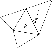
Ansys Icepak stores discrete values of the scalar φ at the cell centers (c0 and c1 in Figure 40.8: Control Volume Used to Illustrate Discretization of a Scalar Transport Equation). However, face values φ_f are required for the convection terms in Equation 40–122 and must be interpolated from the cell center values. This is accomplished using an upwind scheme.

Upwinding means that the face value φ_f is derived from quantities in the cell upstream, or "upwind", relative to the direction of the normal velocity v_n in Equation 40–122. Ansys Icepak allows you to choose from two upwind schemes: first-order upwind, and second-order upwind. These schemes are described below.

The diffusion terms in Equation 40–122 are central-differenced and are always second-order accurate.

First-Order Upwind Scheme

When first-order accuracy is desired, quantities at cell faces are determined by assuming that the cell-center values of any field variable represent a cell-average value and hold throughout the entire cell; the face quantities are identical to the cell quantities. Thus when first-order upwinding is selected, the face value φ_f is set equal to the cell-center value of φ in the upstream cell.

Second-Order Upwind Scheme

When second-order accuracy is desired, quantities at cell faces are computed using a multidimensional linear reconstruction approach  [ 1 ]. In this approach, higher-order accuracy is achieved at cell faces through a Taylor series expansion of the cell-centered solution about the cell centroid. Thus when second-order upwinding is selected, the face value φ_f is computed using the following expression:

(40–123)

where φ and ∇φ are the cell-centered value and its gradient in the upstream cell, and Δs is the displacement vector from the upstream cell centroid to the face centroid. This formulation requires the determination of the gradient ∇φ in each cell. This gradient is computed using the divergence theorem, which in discrete form is written as

(40–124)

Here the face values are computed by averaging φ from the two cells adjacent to the face. Finally, the gradient ∇φ is limited so that no new maxima or minima are introduced.

Linearized Form of the Discrete Equation

The discretized scalar transport equation (Equation 40–122) contains the unknown scalar variable φ at the cell center as well as the unknown values in surrounding neighbor cells. This equation will, in general, be nonlinear with respect to these variables. A linearized form of Equation 40–122 can be written as

(40–125)

where the subscript nb refers to neighbor cells, and a_p and a_nb are the linearized coefficients for φ and φ_b .

The number of neighbors for each cell depends on the grid topology, but will typically equal the number of faces enclosing the cell (boundary cells being the exception).

Similar equations can be written for each cell in the grid. This results in a set of algebraic equations with a sparse coefficient matrix. For scalar equations, Ansys Icepak solves this linear system using a point implicit (Gauss-Seidel) linear equation solver in conjunction with an algebraic multigrid (AMG) method which is described in Restriction, Prolongation, and Coarse-Level Operators.

Under-Relaxation

Because of the nonlinearity of the equation set being solved by Ansys Icepak, it is necessary to control the change of φ. This is typically achieved by under-relaxation, which reduces the change of φ produced during each iteration. In a simple form, the new value of the variable φ within a cell depends upon the old value, φ_old , the computed change in φ, Δφ, and the under-relaxation factor, α , as follows:

(40–126)

Discretization of the Momentum and Continuity Equations

In this section, special practices related to the discretization of the momentum and continuity equations and their solution are addressed. These practices are most easily described by considering the steady-state continuity and momentum equations in integral form:

(40–127)

(40–128)

where is the identity matrix, is the stress tensor, and is the force vector.

Discretization of the Momentum Equation

The discretization scheme described earlier in this section for a scalar transport equation is also used to discretize the momentum equations. For example, the x-momentum equation can be obtained by setting φ = u:

(40–129)

If the pressure field and face mass fluxes were known, Equation 40–129 could be solved in the manner outlined earlier in this section, and a velocity field obtained. However, the pressure field and face mass fluxes are not known a priori and must be obtained as a part of the solution. There are important issues with respect to the storage of pressure and the discretization of the pressure gradient term; these are addressed later in this section.

Ansys Icepak uses a co-located scheme, whereby pressure and velocity are both stored at cell centers. However, Equation 40–129 requires the value of the pressure at the face between cells c0 and c1, shown in Figure 40.8: Control Volume Used to Illustrate Discretization of a Scalar Transport Equation. Therefore, an interpolation scheme is required to compute the face values of pressure from the cell values.

Pressure Interpolation Schemes

The default pressure interpolation scheme in Ansys Icepak is the standard scheme. This scheme interpolates the pressure values at the faces using momentum equation coefficients  [ 21 ]. This procedure works well as long as the pressure variation between cell centers is smooth. When there are jumps or large gradients in the momentum source terms between control volumes, the pressure profile has a high gradient at the cell face, and cannot be interpolated using this scheme. If this scheme is used, the discrepancy shows up in overshoots/undershoots of cell velocity.

Flows for which the standard pressure interpolation scheme will have trouble include flows with large body forces, such as in strongly swirling flows and in high-Rayleigh-number natural convection. In such cases, it is necessary to pack the mesh in regions of high gradient to resolve the pressure variation adequately.

Another source of error is that Ansys Icepak assumes that the normal pressure gradient at the wall is zero. This is valid for boundary layers, but not in the presence of body forces or curvature. Again, the failure to correctly account for the wall pressure gradient is manifested in velocity vectors pointing in/out of walls.

The other scheme available in Ansys Icepak is the body-force-weighted scheme. This scheme computes the face pressure by assuming that the normal acceleration of the fluid resulting from the pressure gradient and body forces is continuous across each face. This works well if the body forces are known a priori in the momentum equations (for example, buoyancy and axisymmetric swirl calculations). This scheme is good for high-Rayleigh-number natural convection flows.

Discretization of the Continuity Equation

Equation 40–127 may be integrated over the control volume in Figure 40.8: Control Volume Used to Illustrate Discretization of a Scalar Transport Equation to yield the following discrete equation

(40–130)

where J_f is the mass flux through face f, ρv_n .

As described in Overview of Numerical Scheme, the momentum and continuity equations are solved sequentially. In this sequential procedure, the continuity equation is used as an equation for pressure. However, pressure does not appear explicitly in Equation 40–130 for incompressible flows, since density is not directly related to pressure. The SIMPLE (Semi-Implicit Method for Pressure-Linked Equations) algorithm  [ 20 ] is used for introducing pressure into the continuity equation. This procedure is outlined below.

To proceed further, it is necessary to relate the face values of velocity v_n to the stored values of velocity at the cell centers. Linear interpolation of cell-centered velocities to the face results in unphysical checker-boarding of pressure. Ansys Icepak uses a procedure similar to that outlined by Rhie and Chow [ 21 ] to prevent checkerboarding. The face value of velocity v_n is not averaged linearly; instead, momentum-weighted averaging, using weighting factors based on the a_P coefficient from Equation 40–129, is performed. Using this procedure, the face flow rate J_f may be written as

(40–131)

where P_c0 and P_c1 are the pressures within the two cells on either side of the face, and Ĵ_f contains the influence of velocities in these cells (see Figure 40.8: Control Volume Used to Illustrate Discretization of a Scalar Transport Equation). The term d_f is a function of ā_P , the average of the momentum equation a_P coefficients for the cells on either side of face f.

Pressure-Velocity Coupling with SIMPLE

Pressure-velocity coupling is achieved by using Equation 40–131 to derive an equation for pressure from the discrete continuity equation (Equation 40–130). Ansys Icepak uses the SIMPLE (Semi-Implicit Method for Pressure-Linked Equations) pressure-velocity coupling algorithm. The SIMPLE algorithm uses a relationship between velocity and pressure corrections to enforce mass conservation and to obtain the pressure field.

If the momentum equation is solved with a guessed pressure field p^∗ , the resulting face flux J_f ^∗ computed from Equation 40–131

(40–132)

does not satisfy the continuity equation. Consequently, a correction J_f ^′ is added to the face flow rate J_f ^∗ so that the corrected face flow rate J_f

(40–133)

satisfies the continuity equation. The SIMPLE algorithm postulates that J_f ^′ be written as

(40–134)

where is the cell pressure correction.

The SIMPLE algorithm substitutes the flux correction equations (Equation 40–133 and  Equation 40–134) into the discrete continuity equation (Equation 40–130) to obtain a discrete equation for the pressure correction p^′ in the cell:

(40–135)

where the source term b is the net flow rate into the cell:

(40–136)

The pressure-correction equation (Equation 40–135) may be solved using the algebraic multigrid (AMG) method described in Restriction, Prolongation, and Coarse-Level Operators. Once a solution is obtained, the cell pressure and the face flow rate are corrected using

(40–137)

(40–138)

Here α _p is the under-relaxation factor for pressure (see Equation 40–126 and related description for information about under-relaxation). The corrected face flow rate J_f satisfies the discrete continuity equation identically during each iteration.

Coupled Pressure-Velocity Formulation

Selecting Coupled pressure-velocity formulation from the Solver options group box indicates that you are using the pressure-based coupled algorithm which is described in this section.

The pressure-based solver allows you to solve your flow problem in either a segregated or coupled manner. Using the coupled approach offers some advantages over the non-coupled or segregated approach. The coupled scheme obtains a robust and efficient single phase implementation for steady-state flows, with superior performance compared to the segregated SIMPLE solution scheme. For transient flows, using the coupled algorithm is necessary when the quality of the mesh is poor, or if large time steps are used.

The pressure-based segregated algorithm solves the momentum equation and pressure correction equations separately. This semi-implicit solution method results in slow convergence.

The coupled algorithm solves the momentum and pressure-based continuity equations together. The full implicit coupling is achieved through an implicit discretization of pressure gradient terms in the momentum equations, and an implicit discretization of the face mass flux, including the Rhie-Chow pressure dissipation terms.

In the momentum equations (Equation 40–129), the pressure gradient for component is of the form

(40–139)

Where is the coefficient derived from the Gauss divergence theorem and coefficients of the pressure interpolation schemes. Finally, for any th cell, the discretized form of the momentum equation for component is defined as

(40–140)

In the continuity equation, the balance of fluxes is replaced using the flux expression in Equation 40–131, resulting in the discretized form

(40–141)

As a result, the overall system of equations (Equation 40–140 and Equation 40–141), after being transformed to the -form, is presented as

(40–142)

where the influence of a cell on a cell has the form

(40–143)

and the unknown and residual vectors have the form

(40–144)

(40–145)

Note that Equation 40–142 is solved using the coupled AMG.

 

40.7.2.1. Pseudo Transient Under-Relaxation

The pseudo transient under-relaxation method is a form of implicit under-relaxation. Here, the under-relaxation is controlled through the pseudo time step size. The pseudo time step size, which is automatically calculated by the solver, can be the same or different for different equations solved.

(40–146)

where is the pseudo time step.