


This section describes the mathematical basis of the multigrid approach used in Ansys Icepak.
Approach
Ansys Icepak uses a multigrid scheme to accelerate the convergence of the solver by computing corrections on a series of coarse grid levels. The use of this multigrid scheme can greatly reduce the number of iterations and the CPU time required to obtain a converged solution, particularly when your model contains a large number of control volumes.
Implicit solution of the linearized equations on unstructured meshes is complicated by the fact that there is no equivalent of the line-iterative methods that are commonly used on structured grids. Because direct matrix inversion is out of the question for realistic problems and "whole-field" solvers that rely on conjugate-gradient (CG) methods have robustness problems associated with them, the methods of choice are point implicit solvers like Gauss-Seidel . Although the Gauss-Seidel scheme rapidly removes local (high-frequency) errors in the solution, global (low-frequency) errors are reduced at a rate inversely related to the grid size. Thus, for a large number of nodes, the solver "stalls" and the residual reduction rate becomes prohibitively low.
Multigrid techniques allow global error to be addressed by using a sequence of successively coarser meshes. This method is based upon the principle that global (low-frequency) error existing on a fine mesh can be represented on a coarse mesh where it again becomes accessible as local (high-frequency) error: because there are fewer coarse cells overall, the global corrections can be communicated more quickly between adjacent cells. Because computations can be performed at exponentially decaying expense in both CPU time and memory storage on coarser meshes, there is the potential for very efficient elimination of global error. The fine-grid relaxation scheme or "smoother", in this case either the point-implicit Gauss-Seidel or the explicit multi-stage scheme, is not required to be particularly effective at reducing global error and can be tuned for efficient reduction of local error.
The Basic Concept in Multigrid
Consider the set of discretized linear (or linearized) equations given by
 | (40–152) |
where φe is the exact solution. Before the solution has converged there will be a defect d associated with the approximate solution φ:
 | (40–153) |
We seek a correction ψ to φ such that the exact solution is given by
 | (40–154) |
Substituting Equation 40–154 into Equation 40–152 gives
 | (40–155) |
Now using Equation 40–153 and Equation 40–155 we obtain
 | (40–156) |
which is an equation for the correction in terms of the original fine level operator A and the defect d. Assuming the local (high-frequency) errors have been sufficiently damped by the relaxation scheme on the fine level, the correction ψ will be smooth and therefore more effectively solved on the next coarser level.
Solving for corrections on the coarse level requires transferring the defect down from the fine level (restriction), computing corrections, and then transferring the corrections back up from the coarse level (prolongation). We can write the equations for coarse level corrections ψH as
 | (40–157) |
where AH is the coarse level operator and R the restriction operator responsible for transferring the fine level defect down to the coarse level. Solution of Equation 40–157 is followed by an update of the fine level solution given by
 | (40–158) |
where P is the prolongation operator used to transfer the coarse level corrections up to the fine level.
The primary difficulty with using multigrid on unstructured grids is the creation and use of the coarse grid hierarchy. On a structured grid, the coarse grids can be formed simply by removing every other grid line from the fine grids and the prolongation and restriction operators are simple to formulate (for example, injection and bilinear interpolation).
Multigrid Cycles
A multigrid cycle can be defined as a recursive procedure that is applied at each grid level as it moves through the grid hierarchy. Four types of multigrid cycles are available in Ansys Icepak: the V, W, F, and flexible ("flex") cycles.
Figure 40.9: V-Cycle Multigrid and Figure 40.10: W-Cycle Multigrid show the V and W multigrid cycles (defined below). In each figure, the multigrid cycle is represented by a square, and then expanded to show the individual steps that are performed within the cycle. You may want to follow along in the figures as you read the steps below.

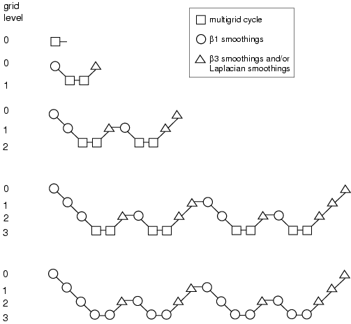
For the V and W cycles, the traversal of the hierarchy is governed by three parameters, β1 , β2 , and β3 , as follows:
β1 "smoothings", (sometimes called pre-relaxation sweeps), are performed at the current grid level to reduce the high-frequency components of the error (local error).
In Figure 40.9: V-Cycle Multigrid and Figure 40.10: W-Cycle Multigrid this step is represented by a circle and marks the start of a multigrid cycle. The high-wave-number components of error should be reduced until the remaining error is expressible on the next coarser mesh without significant aliasing.
If this is the coarsest grid level, then the multigrid cycle on this level is complete. (In Figure 40.9: V-Cycle Multigrid and Figure 40.10: W-Cycle Multigrid there are 3 coarse grid levels, so the square representing the multigrid cycle on level 3 is equivalent to a circle, as shown in the final diagram in each figure.)
Note: In Ansys Icepak, β1 is zero (that is, pre-relaxation is not performed).
Next, the problem is "restricted" to the next coarser grid level using the appropriate restriction operator.
In Figure 40.9: V-Cycle Multigrid and Figure 40.10: W-Cycle Multigrid, the restriction from a finer grid level to a coarser grid level is designated by a downward-sloping line.
The error on the coarse grid is reduced by performing β2 multigrid cycles (represented in Figure 40.9: V-Cycle Multigrid and Figure 40.10: W-Cycle Multigrid as squares). Commonly, for fixed multigrid strategies β2 is either 1 or 2, corresponding to V-cycle and W-cycle multigrid, respectively.
Next, the cumulative correction computed on the coarse grid is "interpolated" back to the fine grid using the appropriate prolongation operator and added to the fine grid solution.
In Figure 40.9: V-Cycle Multigrid and Figure 40.10: W-Cycle Multigrid the prolongation is represented by an upward-sloping line.
The high-frequency error now present at the fine grid level is due to the prolongation procedure used to transfer the correction.
In the final step, β3 "smoothings" (post-relaxations) are performed to remove the high-frequency error introduced on the coarse grid by the β2 multigrid cycles.
In Figure 40.9: V-Cycle Multigrid and Figure 40.10: W-Cycle Multigrid, this relaxation procedure is represented by a single triangle.
For the flexible cycle, the calculation and use of coarse grid corrections is controlled in the multigrid procedure by the logic illustrated in Figure 40.11: Logic Controlling the Flex Multigrid Cycle. This logic ensures that coarser grid calculations are invoked when the rate of residual reduction on the current grid level is too slow. In addition, the multigrid controls dictate when the iterative solution of the correction on the current coarse grid level is sufficiently converged and should thus be applied to the solution on the next finer grid. These two decisions are controlled by the parameters α and β shown in Figure 40.11: Logic Controlling the Flex Multigrid Cycle, as described in detail below. Note that the logic of the multigrid procedure is such that grid levels may be visited repeatedly during a single global iteration on an equation. For a set of 4 multigrid levels, referred to as 0, 1, 2, and 3, the flex-cycle multigrid procedure for solving a given transport equation might consist of visiting grid levels as 0-1-2-3-2-3-2-1-0-1-2-1-0, for example.
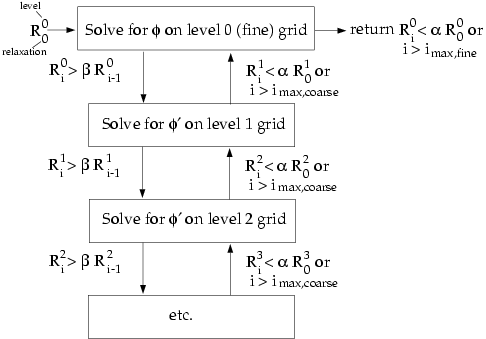
The main difference between the flexible cycle and the V and W cycles is that the satisfaction of the residual reduction tolerance and termination criterion determine when and how often each level is visited in the flexible cycle, whereas in the V and W cycles the traversal pattern is explicitly defined.
The multigrid F cycle is essentially a combination of the V and W cycles described in Multigrid Cycles.
Recall that the multigrid cycle is a recursive procedure. The procedure is expanded to the next coarsest grid level by performing a single multigrid cycle on the current level. Referring to Figure 40.9: V-Cycle Multigrid and Figure 40.10: W-Cycle Multigrid, this means replacing the square on the current level (representing a single cycle) with the procedure shown for the 0–1 level cycle (the second diagram in each figure). We see that a V cycle consists of:
 | (40–159) |
and a W cycle:
 | (40–160) |
An F cycle is formed by a W cycle followed by a V cycle:
 | (40–161) |
As expected, the F cycle requires more computation than the V cycle, but less than the W cycle. However, its convergence properties turn out to be better than the V cycle and roughly equivalent to the W cycle. The F cycle is the default AMG cycle for the coupled equation set and for the scalar energy equation.
The Residual Reduction Rate Criteria
The multigrid procedure invokes calculations on the next coarser grid level when the error reduction rate on the current level is insufficient, as defined by
 | (40–162) |
Here Ri is the absolute sum of residuals (defect) computed on the current grid level after the relaxation on this level. The above equation states that if the residual present in the iterative solution after i relaxations is greater than some fraction, β (between 0 and 1), of the residual present after the (i − 1)th relaxation, the next coarser grid level should be visited. Thus β is referred to as the residual reduction tolerance, and determines when to "give up" on the iterative solution at the current grid level and move to solving the correction equations on the next coarser grid. The value of β controls the frequency with which coarser grid levels are visited. The default value is 0.1. A larger value will result in less frequent visits, and a smaller value will result in more frequent visits.
Provided that the residual reduction rate is sufficiently rapid, the correction equations will be converged on the current grid level and the result applied to the solution field on the next finer grid level.
The correction equations on the current grid level are considered sufficiently converged when the error in the correction solution is reduced to some fraction, α (between 0 and 1), of the original error on this grid level:
 | (40–163) |
Here, Ri is the residual on the current grid level after the ith iteration on this level, and R0 is the residual that was initially obtained on this grid level at the current global iteration. The parameter α , referred to as the termination criterion, has a default value of 0.1. Note that the above equation is also used to terminate calculations on the lowest (finest) grid level during the multigrid procedure. Thus, relaxations are continued on each grid level (including the finest grid level) until the criterion of this equation is obeyed (or until a maximum number of relaxations has been completed, in the case that the specified criterion is never achieved).
Restriction, Prolongation, and Coarse-Level Operators
The multigrid algorithm in Ansys Icepak is referred to as an "algebraic" multigrid (AMG) scheme because, as we shall see, the coarse level equations are generated without the use of any geometry or re-discretization on the coarse levels; a feature that makes AMG particularly attractive for use on unstructured meshes. The advantage is that no coarse grids have to be constructed or stored, and no fluxes or source terms need be evaluated on the coarse levels. This approach is in contrast with FAS (sometimes called "geometric") multigrid in which a hierarchy of meshes is required and the discretized equations are evaluated on every level. In theory, the advantage of FAS over AMG is that the former should perform better for non-linear problems since non-linearities in the system are carried down to the coarse levels through the re-discretization; when using AMG, once the system is linearized, non-linearities are not "felt" by the solver until the fine level operator is next updated.
AMG Restriction and Prolongation Operators
The restriction and prolongation operators used here are based on the additive correction (AC) strategy described for structured grids by Hutchinson and Raithby [ 10 ]. Inter-level transfer is accomplished by piecewise constant interpolation and prolongation. The defect in any coarse level cell is given by the sum of those from the fine level cells it contains, while fine level corrections are obtained by injection of coarse level values. In this manner the prolongation operator is given by the transpose of the restriction operator
 | (40–164) |
The restriction operator is defined by a coarsening or "grouping" of fine level cells into coarse level ones. In this process each fine level cell is grouped with one or more of its "strongest" neighbors, with a preference given to currently ungrouped neighbors. The algorithm attempts to collect cells into groups of fixed size, typically two or four, but any number can be specified. In the context of grouping, strongest refers to the neighbor j of the current cell i for which the coefficient Aij is largest. For sets of coupled equations Aij is a block matrix and the measure of its magnitude is simply taken to be the magnitude of its first element. In addition, the set of coupled equations for a given cell are treated together and not divided amongst different coarse cells. This results in the same coarsening for each equation in the system.
The coarse level operator AH is constructed using a Galerkin approach. Here we require that the defect associated with the corrected fine level solution must vanish when transferred back to the coarse level. Therefore we may write
 | (40–165) |
Upon substituting Equation 40–153 and Equation 40–158 for dnew and φnew we have
 | (40–166) |
Now rearranging and using Equation 40–153 once again gives
 | (40–167) |
Comparison of Equation 40–167 with Equation 40–157 leads to the following expression for the coarse level operator:
 | (40–168) |
The construction of coarse level operators thus reduces to a summation of diagonal and corresponding off-diagonal blocks for all fine level cells within a group to form the diagonal block of that group’s coarse cell.