


Many engine companies are now investigating the technical challenges posed by dual-fuel combustion in engines. Dual-fuel combustion has the advantage of providing diesel-like efficiency with gasoline as the primary fuel, providing potential increases in efficiency of 50% while reducing emissions. Typical dual-fuel combustion designs involve the use of a small pilot injection of a liquid fuel that is relatively easy to ignite. The pilot is injected into a lean mixture of air and a more volatile fuel that is less inclined to autoignite, but which is port-injected to provide good mixing with the air prior to ignition. Diesel is typically used as the pilot and it can be injected in very small amounts, sometimes referred to as micro-pilots. Gasoline is the typical port-injected fuel for transportation applications and natural gas for power applications. Other liquid and gaseous fuels are of interest for power applications such as landfill gas, process gas and refinery gas. Ansys Forte allows the use of accurate fuel models to capture fuel effects of both the ignition and flame propagation processes in a computationally efficient manner.
Ansys Forte uses the well established G-equation model for tracking flame propagation. In spark-ignited engines, flame propagation is initiated by a spark event, using a kernel ignition model. For dual-fuel cases, however, the injection and auto-ignition of the liquid pilot fuel serves to initiate the flame propagation. In Ansys Forte, the simulation can consider both auto-ignition and flame-propagation modes of combustion progress simultaneously. The Ansys Forte auto-ignition mode of initiating flame propagation models takes advantage of a good fuel model's ability to accurately predict ignition under auto-ignition conditions of temperature and pressure. In addition, the flame-propagation model uses a locally calculated turbulent flame-speed that derives from fuel-specific flame-speed calculations using detailed kinetics models. In this way, both auto-ignition and flame-propagation benefit from accurate fuel models for low-temperature and high-temperature kinetics. The details of the autoignition-induced flame propagation model are included in the Ansys Forte Theory Manual.
The Ansys Forte Simulation workflow allows the use of either a body-fitted mesh or an automatically generated mesh. In this tutorial, we will focus on the use of a mesh previously generated using the Sector Mesh Generator.
A sector can represent the full geometry because we can take advantage of the periodicity of injector nozzle-hole pattern and the symmetry of the cylinder. For example, a six-hole injector allows simulation using a 60° sector (360/6). By using the symmetry of the problem in this way, the mesh created is much smaller and the simulation therefore runs faster than it would with a complete 360° mesh.
This tutorial describes the use of 82% premixed gasoline with an 18% liquid diesel pilot for ignition. The tutorial is based upon work previously published that also looks at 78% gasoline and 85% gasoline cases (Puduppakkam et al. 2011, as described in Reference).
The files for this tutorial are obtained by downloading the
dualfuel_gasoline.zip file
here
.
Unzip dualfuel_gasoline.zip to your working folder.
Profile1.csv: Data describing the spray injections. These data can be entered using cut and paste or using the Import option within the Profile Editor tool, which can be opened in the context of the spray-injection panel on the Simulation User Interface.
Dual_Fuels_82percentGasoline_AMG_Tutorial.ftsim: A project file of the completed tutorial, for verification or comparison of your progress in the tutorial set-up.
The sample files are provided as a download. You have the opportunity to select the location for the files when you download and decompress the sample files.
Forte may be launched in a command line mode to perform certain tasks such as preparing a run for execution, importing project settings from a text file, or various other tasks described in the Forte User's Guide. One of these tools allows exporting a textual representation of the project data to a text file.
Example
forte.sh CLI -project <project_name>.ftsim -export tutorial_settings.txt
Briefly, you can double-check project settings by saving your project and then running the command-line utility to export the settings in your tutorial project (<project_name>.ftsim), and then use the command a second time to export the settings in the provided final version of the tutorial. Compare them with your favorite diff tool, such as DIFFzilla. If all the parameters are in agreement, you have set up the project successfully. If there are differences, you can go back into the tutorial set-up, re-read the tutorial instructions, and change the setting of interest.
Note: This tutorial is based on a fully configured sample project that contains the tutorial project settings. The description provided here covers the key points of the project set-up but is not intended to explain every parameter setting in the project. The project files have all custom and default parameters already configured; the text highlights only the significant points of the tutorial.
The project setup workflow follows the top-down order of the workflow tree in the Ansys Forte Simulate interface. The components irrelevant to the present project will not be mentioned in this document, and you can simply skip them and use the default model options.
Note: All Editor panel options that are not explicitly mentioned in this tutorial should be left at their default values. Changed values on any Editor panel do not take effect until you press the Apply button.
The Gasoline-ethanol_4comp_179sp__knocking__soot-pseudo-gas.cks chemistry set from the Forte data directory has been used in this tutorial. This encrypted reduced chemistry has 179 species participating in 1381 reactions and includes reaction pathways for the surrogate components used in this tutorial, n-heptane and iso-octane. In this tutorial, simple 1-component surrogates have been used for diesel (n-heptane) and gasoline (iso-octane). Customized surrogates and corresponding reduced chemistry can be used to better represent the fuels; for simplicity, here we are using simple surrogates and already available reduced chemistry from the Forte data directory.
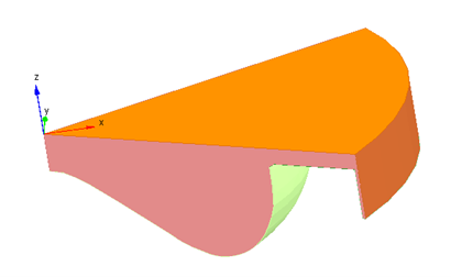
As shown in Figure 3.1: Geometry visualized in Simulate's 3-D View, you can see the sector geometry in the 3-D View window in the center. If you wish, you can rename the geometry elements by right- clicking an element's name. The geometry elements and Boundary Conditions are listed in the Visualization tree on the right, where you can perform many operations such as turning the visibility of the mesh ON and OFF, increasing opacity, changing color, etc., by right-clicking the element.
Under Mesh Controls, the Global mesh size has been set to 2 mm, along with the following refinements:
Surface refinement is used for:
For the piston, head, and liner surfaces. 1 layer of cells of 1 mm (½ of global mesh size) are added to these surfaces. This refinement is always turned ON. This mesh control is used to adequately refine these boundaries.
For the crevice region. 1 layer of cells of 0.25 mm (that is, 1/8th of global mesh size) are added. This refinement is always turned on. This mesh control is used to adequately refine the small crevice geometry.
For the squish region. 2 layers of cells of 0.5 mm (that is, 1/4th of global mesh size) are added. This refinement is turned on from -30 to +30 CA ATDC, and is to ensure the small squish region near TDC is adequately refined.
Line refinement is used for:
Along the sector mesh axis. Over a cylindrical region around the axis with a radius of 1 mm, 0.25 mm cells are used (that is, 1/8th global mesh size). This refinement is to ensure adequate refinement near the sector mesh axis, and is always turned on.
Point refinement is used:
To cover the entire domain with 1 mm cells (that is, ½ of global mesh size) from -20 to +20 CA ATDC. This is to ensure more accurate mesh resolution when ignition and the majority of heat release occurs. This is done by using a large enough (4 cm) radius of application for this point refinement mesh control.
Cone refinement is used for:
Adequately refining the spray path. The refinement is turned on from near SOI of -67 CA ATDC to slightly past expected ignition (10 CA ATDC). The refinement uses cells of 1 mm (that is, ½ of global mesh size).
Solution adaptive meshing is used for:
Gradient of fuel vapor mass fraction, from near SOI -67 CA ATDC to slightly past expected ignition (+10 CA ATDC). 0.5 mm cells (that is, 1/4 global mesh size) are used, to appropriately capture events leading up to combustion of fuel. Statistical bounds are used with a Sigma threshold of 0.5.
Gradient of velocity, from near SOI -67 CA ATDC to slightly past expected ignition (+10 CA ATDC). 0.5 mm cells (that is, 1/4 global mesh size) are used, to appropriately capture spray dynamics. Statistical bounds are used with a Sigma threshold of 0.5.
Gradient of temperature, from near SOI -67 CA ATDC to 50 CA, where most heat release and emissions evolution have occurred. 0.5 mm cells (that is, 1/4 global mesh size) are used, to appropriately capture combustion and emissions evolution. Statistical bounds are used with a Sigma threshold of 0.5.
Now that the meshing options have been set up, you can set up the models and solver options using the guided tasks in the Simulation Workflow tree. In many cases, default parameters are assumed and employed, such that no input is required. The required inputs and changes to the setup panels for this case are described here.
In the Workflow tree, expand Models.
Models > Chemistry: On the Chemistry icon bar, the Import Chemistry
 icon has been used to import the chemistry. This opens a file browser
where you can navigate to and select a chemistry set file. For this project, however, we use a
pre-installed chemistry set that comes with Ansys Forte. The chemistry file
(.cks ) is a standard Ansys Chemkin chemistry-set file.
More information about the chemistry set and the files referenced within it can be found in
the Ansys Forte User
Guide.
icon has been used to import the chemistry. This opens a file browser
where you can navigate to and select a chemistry set file. For this project, however, we use a
pre-installed chemistry set that comes with Ansys Forte. The chemistry file
(.cks ) is a standard Ansys Chemkin chemistry-set file.
More information about the chemistry set and the files referenced within it can be found in
the Ansys Forte User
Guide.Models > Transport: For this node, keep all the default settings.
Models > Spray Model: Since this is a direct-injection case, turn ON (check) Spray Model to display its icon bar (action bar) in the Editor panel. In the panel, keep the defaults. Leave the Use Vaporization Model (default) check ON.
Add an Injector: The icon bar provides two spray-injector options: Hollow Cone or Solid Cone. For the diesel injector, click the Solid Cone
 icon. In the dialog that opens, name the new solid-cone injector as
"Solid Injector". This opens another icon bar and Editor
panel for the new solid-cone injector. In the Editor panel, configure the model parameters
for the solid-cone injector.
icon. In the dialog that opens, name the new solid-cone injector as
"Solid Injector". This opens another icon bar and Editor
panel for the new solid-cone injector. In the Editor panel, configure the model parameters
for the solid-cone injector. Composition: Select Create New... in the Composition drop-down menu under Settings and click the pencil
 icon to open the Fuel Mixture Editor. In the Fuel Mixture panel,
click the Add Species button and select nc7h16
(that is, n-heptane) as the Species,
n-Tetradecane as the Physical Properties and
enter 1.0 as the Mass Fraction. At the bottom of
the panel, you can keep the default name of "Fuel Mixture 1". Click
Save and Close the window.
icon to open the Fuel Mixture Editor. In the Fuel Mixture panel,
click the Add Species button and select nc7h16
(that is, n-heptane) as the Species,
n-Tetradecane as the Physical Properties and
enter 1.0 as the Mass Fraction. At the bottom of
the panel, you can keep the default name of "Fuel Mixture 1". Click
Save and Close the window.Change the Parcel Specification to Droplet Density, and set the Droplet Number Density = 1, its default value.
Set Inflow Droplet Temperature = 360.0 K.
Set Spray Initialization to Discharge Coefficient and Angle, and Discharge Coefficient = 0.8 and Cone Angle = 12.0 degrees.
The Droplet Size Distribution is set to Uniform Size by default.
Under the Solid Cone Breakup Model Settings, leave the KH Model Constants, and RT Model Constants, at their default values, except for the Size constant of RT Breakup (set to 0.1); and RT Distance Constant (set to 1.5). .
Use the Gas Jet Model, with the default parameters.
Click Apply.
Create a Nozzle: While Solid Injector is selected in the Workflow tree, click the New Nozzle
 icon on the icon bar and name the nozzle Nozzle.
"Nozzle" then appears in the Workflow tree, and the Editor panel and icon bar
transform to allow specification of the Nozzle geometry and orientation. Set the parameters
in the Editor panel to:
icon on the icon bar and name the nozzle Nozzle.
"Nozzle" then appears in the Workflow tree, and the Editor panel and icon bar
transform to allow specification of the Nozzle geometry and orientation. Set the parameters
in the Editor panel to: Reference Frame: Select Global Origin from the drop-down menu. For Coord. System = Cylindrical, with R = 0.097 cm, Θ= 30.0 degrees, and A = -0.1 cm.
For Spray Direction, select Spherical from the drop-down menu and then Θ = 107.5 degrees and φ = 0 degrees.
For Nozzle Size, select Area and set Nozzle Area = 0.000491 cm2.
Click Apply. You can see the nozzle appear at the top of the geometry. (You may want to make the Geometry non-opaque or change the color of the nozzle itself by right-clicking in the Workflow tree and selecting Color or Opacity to make the nozzle easier to see in the interior.)
Add an Injection: In the Workflow tree, click Solid Injector again and click the New Injection
 icon on the Solid Injector icon bar and name the
injection "Injection 1". The new Injection item appears in
the Workflow tree, and the Editor panel and the icon bar transform to allow specification of
the injection properties. In the Editor panel, select Crank Angle as
the Timing option and then specify the Start of
injection and Duration of injection as -67.0 and
5.46 degrees, respectively. Accept the default of
Pulsed Injection Type. Set the Total
Injected Mass = 0.015042 g.
icon on the Solid Injector icon bar and name the
injection "Injection 1". The new Injection item appears in
the Workflow tree, and the Editor panel and the icon bar transform to allow specification of
the injection properties. In the Editor panel, select Crank Angle as
the Timing option and then specify the Start of
injection and Duration of injection as -67.0 and
5.46 degrees, respectively. Accept the default of
Pulsed Injection Type. Set the Total
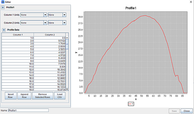
Injected Mass = 0.015042 g. Injection Profile: Click the Create new... option in the profile selection menu next to Velocity Profile, then click the pencil
icon to open the Profile Editor. The new Injection Profile item appears
in the Workflow tree, and the Editor panel and the icon bar transform to the new Injection
Profile. In the Editor panel, make sure all the Units are set to
None for both columns (the dimensionless data is automatically scaled
within Ansys Forte to match the mass and duration of injection) and click the Load
CSV button at the bottom of the panel (you may have to expand the panel size to
see the button). Then navigate to the Profile1.csv
file (see Files Used in This Tutorial).
In the new Import CSV Data dialog that opens, select Comma as the
Column delimiter and turn OFF Read Column Titles
and load the profile file. Alternatively, you can type in the Injection Profile data in the
table on the Editor panel or copy and paste from a spreadsheet or 3rd-party editor. Once the
data are entered, go to Profile Name at the bottom-left of the panel
and name the new profile "Profile1" and click
Save in the Profile Editor and then click Apply in
the Editor panel.
Add a second injection. For the second injection, the start of injection is -32.7 degrees ATDC and the duration of injection is 2.73 CA degrees. Use the same profile as above for this injection by selecting it from the pull-down menu next to Injection Profile. Enter the Total Injected Mass as 0.007521 g.
Under Boundary Conditions in the Workflow tree, specify the boundary conditions in the Editor panels associated with each of the four boundary conditions created by importing the mesh. By default the Wall Model for all of the wall boundaries will be set to Law of the Wall. Leave this default setting as well as the default check box that turns ON heat transfer to the wall.
Boundary Conditions > Piston: Set Piston Temperature = 500.0 K. Turn ON Wall Motion with Motion Type set to Slider Crank.
Stroke = 16.51 cm
Connecting Rod Length = 26.16 cm
Bore = 13.716 cm (this is pre-determined from the mesh)
Accept the defaults of Piston is Offset = unchecked (OFF).
For Reference Frame, accept the default Global Origin and Direction parameters.
For Direction, accept the defaults of X and Y = 0.0 and Z = 1.0 for the direction of piston motion.
Click Apply.
Boundary Conditions > Periodicity: Keep the default Sector Angle = 60 degrees. The periodic boundaries, Periodic A and Periodic B, for this boundary condition are automatically selected, based on the boundary flags contained in the imported mesh.
Boundary Conditions > Head: Set Head Temperature = 500.0 K. Click Apply.
Boundary Conditions > Liner: Set Liner Temperature = 430.0 K. Click Apply.
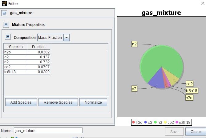
Initial Conditions > Region 1 Initialization (Main): Specify the parameters for the initial conditions as follows:
In the Composition drop-down menu, select Create New... and click the pencil
icon to open the Gas Mixture Editor. In the Gas Mixture panel, click the
Add Species button and select the species in the list indicated in Figure 3.4: Gas Mixture Editor. Once all the species
are entered, provide the values as indicated in Figure 3.4: Gas Mixture Editor. Enter a name for the
Mixture if you desire or leave the default as Mixture
1 in the bottom left text box; click Save, then
Close the window. Temperature = 391.0 K
Pressure = 3.34 bar (note this is not the default unit, so you need to use the pull-down next to the text box to select the correct units option)
In the pull-down menu for the initial Turbulence parameters, select Turbulence Intensity and Length Scale as the way in which we will specify the initial turbulence. For this option we leave the settings with the default values:
Turbulence Intensity Fraction = 0.1 (default value).
Turbulent Length Scale = 1.0 cm (default value).
Velocity is set to Constant.
Select Engine Swirl in the Velocity pull-down and then specify the swirl profile parameters:
Initial Swirl Ratio = -0.7
Initial Swirl Profile Factor = 3.11
Initialize Velocity Components Normal to Piston = ON (checked)
Piston Boundary: Move Piston to the Selected list.
Also keep other options at their defaults.
Click Apply in the Region 1 Initialization Editor panel.
In the Silulation Controls panel, under Simulation Limits, for the Simulation End Points, specify:
Crank Angle Based
Initial Crank Angle = -95.0
RPM = 1,300.0
Cycle Type is 4-Stroke.
Final Simulation Crank Angle = 130.0 degrees. (These two angles correspond to Intake Valve Open and Exhaust Valve Closing, respectively.) Click Apply.
Simulation Controls > Time Step:
Maximum Time Step Option = Constant and enter the value 2.0E-5 sec. (This value is selected so the tutorial example will run fast; the default value is 5.0E-6.)
Leave other settings at their defaults. Click Apply.
Simulation Controls > Chemistry Solver:
Accept the default state of ON (check) for Use Dynamic Cell Clustering and accept its defaults.
Check the option for Use Autoignition-Induced Flame Propagation Model. Use the default values of 2000 K for Critical temperature, and 1 for Critical size coefficient.
Set the Activate Chemistry drop-down menu to Conditionally, specifying After Fuel Injection Starts, and Threshold temperature of 600 K. Click Apply.
Note: More details about the chemistry solver options, such as Dynamic Cell Clustering and Dynamic Adaptive Chemistry, are available in the Ansys Forte User Guide.
Output Controls > Spatially Resolved: For the Spatially Resolved Output Control, specify:
Crank Angle Output Control.
Output every = 5.0 degrees, with additional user-defined crank angle output option for additional outputs near spray injection, ignition and combustion events.
For Spatially Resolved Species, move all the fuel-related and emissions species, such as these, to the Selection list: nc7h16, o2, co2, h2o, co, no, and ic8h18. Click Apply.
Output Controls > Spatially Averaged:
For the Spatially Averaged Output Control, select the Crank Angle option and specify Output Every = 0.5 degree.
For Spatially Averaged Species, select o2, co2, co, no, nc7h16, ic8h18, n2, and h2o, and move all species to the Selection list. Click Apply.
Output Controls > Restart Data: In the Workflow tree, check the box for Restart Data and then in the Restart panel, check the box that says, Write Restart File at Last Simulation Step. Uncheck (turn OFF) any other boxes on the panel. Click Apply.
In the Workflow tree, click the Run Simulation node to open the run control interface.
Click the green arrow "play" button under Start/Save to start the case running. The Status changes to "Running."
To interrupt the run, click the red button under Stop. Then the Status becomes "Stopped".
To start over or restart, first select the file from which you want to start, by clicking on the Browse button in the Run row. Once an appropriate ftrst file is selected, click the green Start again.
The progress of the simulation can be monitored during a run. To monitor the averaged value of simulation variables, click the Monitor Runs
 icon in the Run Simulation icon bar. A new window will appear, with a list
of variables that can be plotted on the left panel in the window. To select one or more
variables to plot, check the boxes in front of them in the Monitor Data panel.
icon in the Run Simulation icon bar. A new window will appear, with a list
of variables that can be plotted on the left panel in the window. To select one or more
variables to plot, check the boxes in front of them in the Monitor Data panel.
Note: To change the units of the plotted variables, go back to the Simulation Interface, Edit on the ribbon or menu and choose Edit Preferences. In the Preferences panel, select the units desired. The next time the Monitor window updates the plots, it will automatically reflect these updated unit preferences.
When a run is finished, the Status becomes Complete in the Run panel of the main Simulate User Interface window. In the Editor panel, we choose Ansys EnSight to post-process the results.
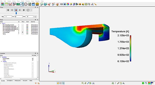
We are interested in creating some average line plots for Pressure, Apparent Heat Release Rate (Apparent HRR) and emissions such as CO vs. Crank Angle. The EnSight view when you read in the Nominal.ftind file is shown in Figure 3.5: Simulation result in EnSight. The thermo.csv file is used to create line plots for Pressure, Apparent HRR, UHC, and CO.
This case models the engine experiment from the following paper:
Karthik V. Puduppakkam, Long Liang, Chitralkumar V. Naik, Ellen Meeks, Sage L. Kokjohn and Rolf D. Reitz, "Use of Detailed Kinetics and Advanced Chemistry-Solution Techniques in CFD to Investigate Dual-Fuel Engine Concepts", SAE International Journal of Engines, Vol. 4, No. 1, pp. 1127-1149, 2011.