Accurately capturing fuel injection, spray breakup and spray vaporization are important aspects of engine-design simulations for direct-injection engines. However, it is difficult to isolate the effects of spray behavior in a full engine simulation involving combustion, moving boundaries and complex turbulent flow. Spray bomb experiments are an excellent method for isolating the spray behavior prior to engine design and analysis. A spray bomb is a quiescent environment where liquid is injected without any moving boundaries, such that the spray characteristics can be examined in detail. Any engine simulation involving liquid injection must account for the key aspects of atomization such as liquid-jet breakup, droplet formation, secondary breakup, droplet collisions, droplet coalescence and vaporization. This tutorial describes how to use Ansys Forte in spray bomb simulations that account for all of these phenomena.
The files for this tutorial are obtained by downloading the
spray_chamber.zip file
here
.
Unzip spray_chamber.zip to your working folder.
Evaporating_Spray_Tutorial.fmsh: This is an Ansys Forte body-fitted mesh file. This file will provide the spray bomb geometry for this Automatic Mesh Generator (AMG) tutorial.
Evaporating_Spray_Tutorial.ftsim: A project file of the completed tutorial, for verification or comparison of your progress in the tutorial set-up.
The tutorial sample files are provided as a download. You have the opportunity to select the location for the files when you download and unzip or untar the sample files.
Note: This tutorial is based on a fully configured sample project that contains the tutorial project settings. The description provided here covers the key points of the project set-up but is not intended to explain every parameter setting in the project. The project files have all custom and default parameters already configured; the text highlights only the significant points of the tutorial.
Forte may be launched in a command line mode to perform certain tasks such as preparing a run for execution, importing project settings from a text file, or various other tasks described in the Forte User's Guide. One of these tools allows exporting a textual representation of the project data to a text file.
Example
forte.sh CLI -project <project_name>.ftsim -export tutorial_settings.txt
Briefly, you can double-check project settings by saving your project and then running the command-line utility to export the settings in your tutorial project (<project_name>.ftsim), and then use the command a second time to export the settings in the provided final version of the tutorial. Compare them with your favorite diff tool, such as DIFFzilla. If all the parameters are in agreement, you have set up the project successfully. If there are differences, you can go back into the tutorial set-up, re-read the tutorial instructions, and change the setting of interest.
For solid-cone spray injections, Ansys Forte utilizes the Kelvin-Helmholtz/Rayleigh-Taylor (KH-RT) spray-breakup models that have been proven to be accurate over a wide range of direct-injection conditions. Together with the gas-jet model, which provides accurate gas-jet entrainment calculations without requiring mesh refinement around the spray, the Ansys Forte spray model provides results that are insensitive to mesh resolution or simulation time step. These spray model components are described in detail in the Ansys Forte Theory Manual.
In many cases, the starting point for a spray injection specification is an estimate of the nozzle discharge coefficient and spray-cone angle. Ansys Forte's nozzle-flow model can optionally provide initial conditions for the spray model by including detailed calculation of the nozzle-flow including cavitation effects.
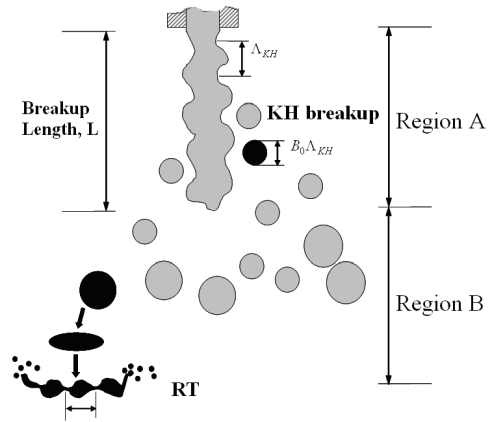
The droplet breakup model consists of two key models. The KH breakup model is applied within the breakup length (see Figure 4.1: KH-RT spray model definitions.). The RT model is then used further downstream with the KH model to predict secondary breakup. The unsteady gas-jet model effectively removes mesh dependency by calculating the gas velocity in the spray region using an analytical model.
Ansys Forte allows you to set several constants that control the initial breakup in the KH region and the secondary breakup in the RT region. Defaults for these constants are provided in Ansys Forte that have been determined after extensive validation with experimental data and should be used initially. However, there could be some cases where an adjustment in these constants would prove useful. The following table describes the specific spray constant name, its default value, a suggested range of adjustment and what the constant controls.
Table 4.1: Description of default Ansys Forte spray constants.
|
Size Constant of KH Breakup |
1.0 |
0.5 - 2.0 |
Affects radius of new droplets formed from initial breakup. |
|
Time Constant of KH Breakup |
40 |
10 - 80 |
Most important constant for controlling spray penetration length. |
|
Critical Mass Fraction for New Droplet Generation |
0.03 |
N/A |
Determines fraction at which new droplets can leave their parent parcel. |
|
Size Constant of RT Breakup |
0.15 |
0.1 - 0.3 |
Affects the radius of the secondary droplets arising from the catastrophic breakup of the parent droplet |
|
Time Constant of RT Breakup |
1.0 |
0.5 - 2.0 |
Affects the characteristic time required to break the parent droplet |
|
RT Distance Constant |
1.9 |
1.5 - 3.0 |
Affects the initial breakup length when the RT model is initiated |
This tutorial considers a cylindrical chamber with no moving walls and quiescent gas (see Table 4.2: Spray bomb simulation case set-up and test conditions.). In this case, pure n-heptane is injected into the chamber. This single component fuel is injected from a single solid-cone injector, where the nozzle hole is located on the wall and the injection is directed towards the center of the chamber. The initial gas in the chamber is a blend of N2, CO2, and H2O, such that the mixture is non-reacting. As the intention of this example is to represent diesel-fuel injection, we use the physical properties of n-tetradecane to represent the fuel. This combination of chemistry model being represented by one fuel surrogate (in this case, n-heptane) while the physical model is represented by another fuel surrogate (in this case, n-tetradecane) is an approach often taken in simulating diesel engine combustion. In this way, the spray-bomb simulation comparisons to experiment can be used to verify the behavior of the surrogate model approach as it will be used in a combustion simulation. For this case, a square injection profile is used. Chemistry calculations are effectively stopped by setting the chemistry solver to begin at a temperature that will not be reached during the simulation.
This tutorial shows the use of the Automatic Mesh Generator. We import a previously generated mesh to provide the spray bomb geometry and select the option upon import to only import the geometry surfaces for use with Automatic Mesh Generation. Mesh sizes of 1 mm, 2 mm, and 3 mm are then used to test mesh dependency. Results for penetration length of the three different mesh sizes are compared against experimental data from SAE Technical Paper 960034 by J.D. Naber and D.L. Siebers [1].
Note: All Editor panel options that are not explicitly mentioned in this tutorial should be left at their default values. Changed values on any Editor panel do not take effect until you press the Apply button.
Table 4.2: Spray bomb simulation case set-up and test conditions.
|
Parameter |
Evaporating Spray Case |
|---|---|
|
Mesh |
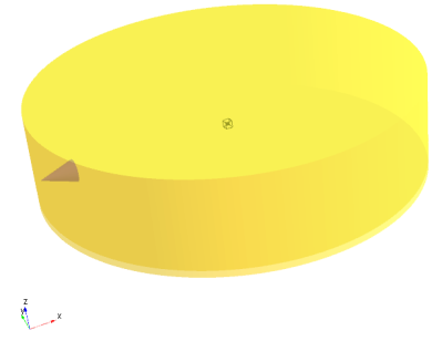
Disc-shaped constant-volume combustion chamber with 114.3 mm diameter and 28.6 mm thickness
|
|
Fuel Type |
Diesel DF2 (Experiment)Tetradecane (Surrogate) |
|
Fuel Temperature |
436 K |
|
Injection Pressure |
1,370 bar |
|
Injection Duration |
4 ms |
|
Nozzle Diameter |
257 μm |
|
Chamber Conditions |
Ta= 1,000 K |
The project setup workflow follows the top-down order of the workflow tree in the Ansys Forte Simulate interface. The components irrelevant to the present project will not be mentioned in this document, and you can simply skip them and use the default model options.
In this tutorial, we will import an existing structured mesh with a size of 2 mm. Mesh sizes of 1 mm, 2 mm, and 3 mm will be investigated to demonstrate mesh independence of the solution. The spray bomb geometry and test conditions are shown in Table 4.2: Spray bomb simulation case set-up and test conditions..
Import the mesh using Geometry on the Workflow tree. Click the Import Geometry
 icon. In the dialog, select Body-fitted mesh in the
drop-down menu, click OK and then navigate to the
Evaporating_Spray_Tutorial.fmsh file in the
location where you saved the downloaded sample files. In the Import
Options window that opens, select Import surface mesh only (use automatic
meshing).
icon. In the dialog, select Body-fitted mesh in the
drop-down menu, click OK and then navigate to the
Evaporating_Spray_Tutorial.fmsh file in the
location where you saved the downloaded sample files. In the Import
Options window that opens, select Import surface mesh only (use automatic
meshing).The imported file displays in the 3-D View area, but may not be ideally zoomed or centered. Click the Refit
 icon to center and resize the mesh.
Mesh Controls: Under Mesh Controls, the Material Point needs to be set to a location that will always be "inside" the boundaries and should be located at least one unit cell length away from any boundaries. To see the coordinate values, select Geometry > Solid.1 in the left-hand Workflow tree. The Editor panel below will show the min/max coordinates. From here we can see that the minimum and maximum coordinate values are –5.714 and 5.714 cm for x- and y-axes, and 0 and 2.86 cm for the z-axis. So, return to Mesh Controls > Material Point, and in the Location options, set X=1 cm, Y=2 cm and Z=1 cm, and click Apply. Once it is set, you can see the Material Point in the 3-D View panel (as a small cube) and it can be made visible/invisible by right-clicking in the Workflow tree and selecting Visibility or Opacity, under Mesh Controls. (You may need to adjust the opacity of the Solid.1 Geometry item as well.)
In the Workflow tree, under Mesh Controls, set the Global Mesh Size to 0.2 cm. This will set the default size of cells to be 2 mm long on each side of the cell cube. Click Apply.
Note: This is within the recommended mesh range; a coarser setting of 0.3 cm could be used for tutorial purposes to produce a shorter runtime.
Click the Mesh Controls node in the Workflow tree. In the icon bar, click the New Surface Refinement Depth
 icon and name the new control "Surfacedepth". (This indicates
that along the selected surface, cells of this smaller size will be used.) A new SurfaceDepth
item appears under Mesh Controls in the Workflow tree. In the panel that appears, select the
Solid.1 surface from the Location list, set the mesh Size as
Fraction of Global Size to 1/2 with an extension of
1 layer. Click Apply.
icon and name the new control "Surfacedepth". (This indicates
that along the selected surface, cells of this smaller size will be used.) A new SurfaceDepth
item appears under Mesh Controls in the Workflow tree. In the panel that appears, select the
Solid.1 surface from the Location list, set the mesh Size as
Fraction of Global Size to 1/2 with an extension of
1 layer. Click Apply.Click the Solution Adaptive Meshing
 icon on the Mesh Controls Editor panel and name the new control
SAM-Velocity. In the Editor panel, set the Quantity Type =
Gradient of Solution Field and Solution Variables = VelocityMagnitude.
Bounds = Statistical and Sigma Threshold = 0.5. Set the
Size as Fraction of Global Size = 1/4. The refinement is Active
= Always, and the Location option is Entire
Domain. Click Apply.
icon on the Mesh Controls Editor panel and name the new control
SAM-Velocity. In the Editor panel, set the Quantity Type =
Gradient of Solution Field and Solution Variables = VelocityMagnitude.
Bounds = Statistical and Sigma Threshold = 0.5. Set the
Size as Fraction of Global Size = 1/4. The refinement is Active
= Always, and the Location option is Entire
Domain. Click Apply.
Chemistry: After the mesh, the models are chosen.
Chemistry is set with Models > Chemistry/Materials. Click the Import
Chemistry ![]() icon and import
Diesel_1comp_35sp.cks from the installed Ansys Forte
data directory. An option is provided to view the
chemistry details such as chemistry source, pre-processing log, gas phase input, gas phase
output, thermodynamic input, transport input and transport output. Note that in this case, the
chemistry is effectively turned off, so the main reason to import the chemistry set is to obtain
the chemical species nc7h16 that will represent the fuel and
n2 for the gas in the chamber.
icon and import
Diesel_1comp_35sp.cks from the installed Ansys Forte
data directory. An option is provided to view the
chemistry details such as chemistry source, pre-processing log, gas phase input, gas phase
output, thermodynamic input, transport input and transport output. Note that in this case, the
chemistry is effectively turned off, so the main reason to import the chemistry set is to obtain
the chemical species nc7h16 that will represent the fuel and
n2 for the gas in the chamber.
Transport: The default RNG k-Ε model turbulence settings are used in this tutorial. Those are specified in the Editor panel for Models > Transport > Turbulence. The default fluid properties are also used, which are in Models > Transport.
Spray Model: To set up the spray model, turn ON (check-mark) Models > Spray Model. First, choose the global Spray Properties, which include using the Adaptive Collision Mesh Model. Also check Use Vaporization Model to include the effects of vaporization, since this case is into a relatively hot gas, where vaporization will occur.
Create Injector: Add a solid-cone spray injector through the Models > Spray Model panel, by clicking on the Solid Cone Spray Injector
 icon. Name the injector (Injector) and configure the
injector and its fuel. In the Injector Editor panel, select Create New...
in the Composition drop-down menu and click the pencil
icon. Name the injector (Injector) and configure the
injector and its fuel. In the Injector Editor panel, select Create New...
in the Composition drop-down menu and click the pencil  icon to open the Fuel Mixture Editor. In the Fuel Mixture panel, click the
Add Species button and select nc7h16 (that is,
n-heptane) as the Species,
n-Tetradecane as the Physical Properties, and
1.0 as the Mass Fraction (Note that you must press
ENTER after entering the values in the table). At the bottom of the panel, type a name such as
"Fuel mixture 1". Click Save and
Close the window.
icon to open the Fuel Mixture Editor. In the Fuel Mixture panel, click the
Add Species button and select nc7h16 (that is,
n-heptane) as the Species,
n-Tetradecane as the Physical Properties, and
1.0 as the Mass Fraction (Note that you must press
ENTER after entering the values in the table). At the bottom of the panel, type a name such as
"Fuel mixture 1". Click Save and
Close the window.Using an Injection Type of Pulsed Injection, change the Parcel Specification to Number of Parcels, then set Injected Parcel Count = 30,000.
Set Inflow Droplet Temperature = 436.0 K.
Set Spray Initialization to Discharge Coefficient and Angle, and Discharge Coefficient = 0.78, and Cone Angle = 19.04 degrees.
Keep default values for Droplet Size Distribution and, under the Solid Cone Breakup Model Settings, for the KH Model Constants, RT Model Constants, and Use Gas-Jet Model. Click Apply.
Next we will add the nozzle and specify the injection parameters under this new injector (see Table 4.4: Nozzle settings and Table 4.5: Injection settings.).
Table 4.3: Injector Settings
|
Parameter |
Setting |
|---|---|
|
Injected Spray Parcels |
30,000 |
|
Inflow Droplet Temperature |
436.0 K |
|
Spray Initialization |
Discharge Coefficient and Angle |
|
Discharge Coefficient |
0.78 |
|
Cone Angle |
19.04 |
Create a Nozzle: Click the New Nozzle
 icon on the Injector icon bar and name the nozzle
"Nozzle". The Nozzle item then appears in the Workflow tree,
and the Editor panel and icon bar transform to allow specification of the Nozzle geometry and
orientation. Set the parameters in the Editor panel to use the Reference
Frame parameters to specify the nozzle location and direction. Keep the
Global Origin and use the following settings:
icon on the Injector icon bar and name the nozzle
"Nozzle". The Nozzle item then appears in the Workflow tree,
and the Editor panel and icon bar transform to allow specification of the Nozzle geometry and
orientation. Set the parameters in the Editor panel to use the Reference
Frame parameters to specify the nozzle location and direction. Keep the
Global Origin and use the following settings:If you cannot see the nozzle in the 3-D View, you may need to adjust the opacity or color choice of the nozzle or the boundary conditions that may be blocking your view of it. Select the desired item in the Visualization tree (on the right side) and right-click to turn ON/OFF visualization, change opacity levels, or change the color assigned to that item.
Create an Injection: In the Workflow tree, click Injector again and click the New Injection
 icon on the Injector icon bar and name the injection
Injection. The new Injection item appears in the Workflow tree, and the
Editor panel and the icon bar transform to allow specification of the injection properties. In
the Editor panel, use the following settings:
icon on the Injector icon bar and name the injection
Injection. The new Injection item appears in the Workflow tree, and the
Editor panel and the icon bar transform to allow specification of the injection properties. In
the Editor panel, use the following settings: Table 4.5: Injection settings.
Parameter
Setting
Timing Option
Time
Start
0.0 sec
Duration
0.004 sec
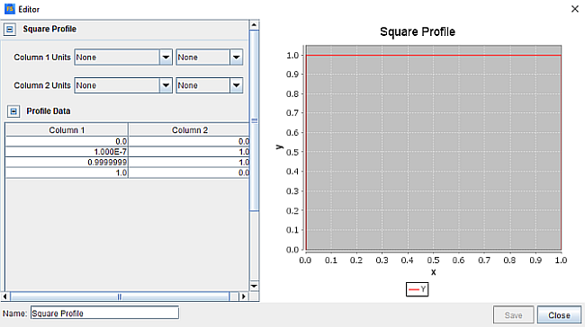
Velocity Profile
Square Profile
Total Injected Mass
0.058 g
The resulting injection profile can be viewed by clicking the pencil ![]() icon next to the Velocity Profile entry box. In this
window, you can also import a new velocity profile for the injection from a
.csv file or make edits directly in the table (see
Figure 4.2: View injection profile).
icon next to the Velocity Profile entry box. In this
window, you can also import a new velocity profile for the injection from a
.csv file or make edits directly in the table (see
Figure 4.2: View injection profile).
Create a new boundary by right-clicking on the Boundary Conditions Workflow tree, and Add a Wall. Now, under the Boundary Conditions Workflow tree node, a new entry called Wall will be found. For this Wall boundary condition, select the Solid.1 surface from the Location list, the No Slip model for handling the boundary layer near the wall, and keep Heat Transfer checked (ON). Set the Thermal Boundary Condition = Wall Temperature, Constant and Temperature = 451 K. Click Apply.
Initial conditions will be set only for the Default Initialization region. Specify the parameters for the initial conditions as follows:
Composition: Select Create new gas mixture... in the Composition drop-down menu and click the pencil
icon to open the Gas Mixture Editor. In the Gas Mixture Editor, select
Composition = Mole Fraction, then click the
Add Species button and select h2o,
co2 and n2 to add. When these 3 species are in the
Species column in the Composition table, enter
0.9033 for the n2 Fraction,
0.0611 for co2 and 0.0356 for
h2o. Name this Gas Mixture 1 in the text field at
the bottom of the Gas Mixture window. Click Save and close the
window.Temperature = 1,000.0 K.
Pressure = 83.04 atm.
In the drop-down menu for the Turbulence parameters, select Turbulence Intensity and Length Scale as the way in which we will specify the initial turbulence. For this option we provide an explicit value for the initial turbulence intensity, but use a length-scale approximation to determine the turbulence dissipation energy. Use these values:
Turbulence Intensity Fraction = 0.0.
Turbulent Length Scale = 1.0 cm.
Select Velocity Components in the Velocity drop-down menu and then specify the velocity components, using the default Reference Frame with Global Origin and Cartesian coordinates set at 0.0, 0.0, 0.0.
Click Apply in this panel.
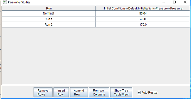
To create a parameter study on pressure, click the Parameter Study  icon next to the Pressure setting (at 83.04 atm). In
the resulting dialog, change the specification to From End Points, set
these values: First run value (A) 40.0, Last run value (B)
170.0, Number of runs (n) 2. Click OK.
icon next to the Pressure setting (at 83.04 atm). In
the resulting dialog, change the specification to From End Points, set
these values: First run value (A) 40.0, Last run value (B)
170.0, Number of runs (n) 2. Click OK.
Close or minimize the Parameter Studies window. Note that the Pressure label in the Editor panel is now blue to indicate that it is associated with a parameter study.
When this simulation runs, a run will occur at each of these pressure settings. See Simulation Results to see how the results vary with the changes in pressure.
Simulation controls allow you to define the simulation limits, time step, chemistry solver and transport terms.
Simulation Limits: Select the Simulation Controls node and then select Time-based for Simulation End Point Option to select a simulation with a Max. Simulation Time of 0.004 sec. Click Apply.
Time Step: In Simulation Controls > Time Step, set the Initial Simulation Time Step to 5.0E-7 sec and use a Constant Max. Time Step Option of 5.0E-6 sec. Advanced Time Step Control Options can be left at the default settings. Click Apply.
Output controls determine what data are stored for viewing during the simulation and for creating plots, graphs and animations.
Spatially Resolved: Set the Output Timing Control = Time and check (turn ON) Interval Based Output Control, set to reporting every 0.0004 sec. To create the Spatially Resolved Species list, be sure to move nc7h16 to the Selection list. Also move n2, co2, and h2o.
Spatially Averaged And Spray: Set the Spatially Averaged Output Control = Time, set to reporting every 4.0E-5 sec. To create the Spatially Averaged Species list, be sure to move nc7h16 to the Selection list. Also move co2, o2, and n2. Click Apply.
Restart Data: Clear (uncheck) the option Write Restart File at Last Simulation Step. Click Apply.
The settings here depend on the system and environment for your simulations. The default for the Run Settings panel is to have nothing selected.
Run Options: Under Job Script Options, change Default Run Type to Parallel and change the default MPI Arguments to 8. (If you do not have MPI installed and configured, keep the default of a serial run.)
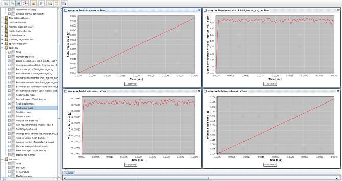
All that is needed to be done now is to select the Nominal run under Run Simulation in the Workflow tree and click the blue arrow Start button. You can monitor the results by clicking on the Monitor icon. In the Monitor window that opens, you can select which result you want to monitor for the spray such as Mass Injected and Penetration Length.
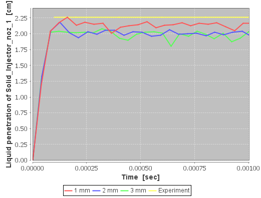
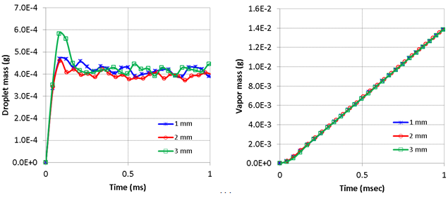
This spray bomb case was run with three mesh sizes (1 mm, 2 mm, and 3 mm) and then compared against experimental data from Naber and Siebers 1. The experimental data provided consisted of penetration depth for the test spray. The experimental data show a penetration depth of 22.6 mm as is shown in Figure 4.5: Mesh sensitivity on spray penetration depth. The simulation results show good agreement with the spray penetration depth as is also seen in Figure 4.5: Mesh sensitivity on spray penetration depth. It is important to note that Ansys Forte defines the spray penetration depth that captures 95% of the liquid. These results also show that the spray is relatively insensitive to the mesh for the three mesh sizes considered. The 1 mm and 2 mm results lie on top of each other. The diversion of the results for 3 mm, suggest that size is a little too large to resolve the fluid mechanics overall and so for these types of cases we would recommend the 2 mm resolution. However, even the coarse mesh results are not far from the resolved-mesh solution, which is an important feature of the Ansys Forte simulations. Another interesting feature is to look at the how the droplet mass and vapor mass evolve during the simulation time. These results are shown in Figure 4.6: Mesh sensitivity on droplet mass and vapor mass, where the mesh is also shown to be insensitive to the mesh size, even with the coarsest mesh. Visualization of the spray results are shown in Figure 4.7: Spray bomb penetration for 2 mm mesh at time = 0.0015 sec.
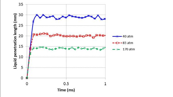
The results of the automated parameter study on ambient pressure in the spray bomb are shown as Figure 4.8: Results of automated parameter study on ambient pressure in the spray bomb. The spray penetration is decreased as the ambient pressure increases due to the increased chamber gas density and drag.
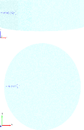
Figure 4.9: Fuel vapor mass fraction distribution for the three different cases shows the fuel vapor mass fraction distribution.
The following Show-Me animation is presented as an animated GIF in Forte's online documentation at the Ansys Help website. If you are reading the PDF version of this manual and want to see the animated GIF, access this section in that online documentation. The interface shown may differ slightly from that in your installed product.