


For diesel engines, the engine combustion is often simulated from intake valve closure (IVC) to exhaust valve opening (EVO), rather than modeling the full air intake or exhaust flow processes involving the intake and exhaust ports, respectively. This is usually a reasonable approximation since the gas in the cylinder at IVC is a relatively homogeneous mixture of air and exhaust gas (due to internal residual or from exhaust-gas recycling), prior to fuel injection. Furthermore, the nozzle hole pattern of the fuel injection usually gives rise to a periodic symmetry, based on the number of nozzle holes. In this tutorial we describe the use of a sector mesh that takes advantage of such symmetry for simulating a diesel engine operating in low-temperature-combustion (LTC) mode. The LTC mode involves an early injection timing, relative to more conventional diesel operation.
A sector can represent the full geometry, since we can take advantage of the periodicity of the cylinder and injector nozzle-hole pattern. For example, an eight-hole injector allows simulation using a 45° sector (360/8). By using the symmetry of the problem in this way, the mesh created is much smaller and the simulation therefore runs faster than it would with a 360° mesh. Such a simplification usually cannot be made for spark-ignited engine cases due to asymmetries introduced by spark plugs, piston shape, and possibly intake ports.
The files for this tutorial are obtained by downloading the
diesel_sector_mesh.zip file
here
.
Unzip diesel_sector_mesh.zip to your working folder.
sandia_bowl_profile.csv: Data describing the piston bowl shape. This profile can be imported or manually entered in the Profile Editor for use by the Sector Mesh Generator to define the bowl shape.
InjectionProfile.csv: Data describing the spray injection. The data can be imported from this file through the User Interface or manually entered once you reach the Spray node on the Workflow tree through use of the Profile Editor.
UserCrankAngleOutputs.csv: Table of data that contains crank angles going from -22 to +20.
Sandia_Engine_LTC_EarlyInj.ftsim: A project file of the completed tutorial, for verification or comparison of your progress in the tutorial set-up.
The sample files are provided as a download. You have the opportunity to select the location for the files when you download and uncompress the sample files.
Note: This tutorial is based on a fully configured sample project that contains the tutorial project settings. The description provided here covers the key points of the project set-up but is not intended to explain every parameter setting in the project. The project files have all custom and default parameters already configured; the text highlights only the significant points of the tutorial.
Forte may be launched in a command line mode to perform certain tasks such as preparing a run for execution, importing project settings from a text file, or various other tasks described in the Forte User's Guide. One of these tools allows exporting a textual representation of the project data to a text file.
Example
forte.sh CLI -project <project_name>.ftsim -export tutorial_settings.txt
Briefly, you can double-check project settings by saving your project and then running the command-line utility to export the settings in your tutorial project (<project_name>.ftsim), and then use the command a second time to export the settings in the provided final version of the tutorial. Compare them with your favorite diff tool, such as DIFFzilla. If all the parameters are in agreement, you have set up the project successfully. If there are differences, you can go back into the tutorial set-up, re-read the tutorial instructions, and change the setting of interest.
The project setup workflow follows the top-down order of the workflow tree in the Ansys Forte Simulate interface. The components irrelevant to the present project will not be mentioned in this document, and you can simply skip them and use the default model options.
The Ansys Forte Sector Mesh Generator provides six different sample mesh topologies for different piston bowl shapes. The shape of the piston bowl determines which mesh topology is most appropriate. The overview of the process is:
Specify the bowl profile.
Enter engine parameters, such as bore, stroke, etc.
Select a topology for meshing.
Specify the control point locations for the mesh topology if necessary (for Topology 3, these are assumed and the profile must have exactly 3 points to define them).
Specify the number of cells between control points for the mesh.
Generate the mesh and import into Ansys Forte.
Note: All Editor panel options that are not explicitly mentioned in this tutorial should be left at their default values. Changed values on any Editor panel do not take effect until you press the Apply button.
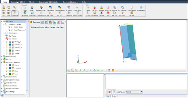
To begin creating a sector mesh, go to the Workflow tree and click Geometry. This opens the Geometry icon bar. Click the Launch Sector Mesh Generator
 icon to open the Sector Mesh Generator Utility (SMG).
Start by clicking the Engine Parameters node in the SMG Project tree to open an Editor panel.
In that panel, the first step is to import the simple bowl profile that was provided with the sample. To do this, go to the Bowl Profile drop-down menu and select Create New... and click the Pencil
 icon. This opens the Profile Editor window.
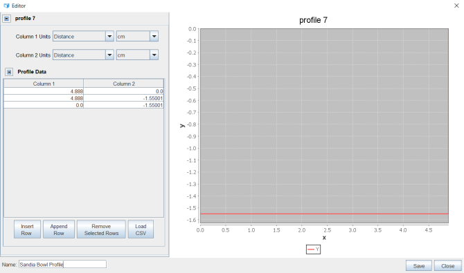
 In the Profile Editor, click the Load CSV button (you may need to expand the window vertically to see the button below the table) and then browse to, select, and open the sandia_bowl_profile.csv file. In the dialog, select Comma as the Column Delimiter and uncheck (turn OFF) the Read Column Titles box and click OK.
In the .csv file, the first column is the X-coordinate and the second column is the Z-coordinate. For this example the "bowl" is completely flat and the wall of the bowl is vertical. For this very simple geometry, only three coordinate points are needed to define the bowl. The profile should look like a flat line in the Profile Editor display, as shown in Figure 2.3: Diesel sector sample mesh as generated in the Sector Mesh Generator. . At the bottom of the Profile Editor panel in the text entry field under Profile Name, enter a name for the profile, such as "Sandia Bowl Profile". See Figure 2.1: Sector Mesh Generator Utility with New Profile and Editor panel . Click Save and Close the window.
Ensure the newly created Sandia Bowl Profile is selected in the Bowl Profile drop-down menu. Next, in the Sector Mesh Generator, specify the engine parameters, which are:
Sector Angle = 45 degrees
Bore = 13.97 cm
Stroke = 15.24 cm
Squish = 0.56 cm
Crevice Width = 0.167 cm
Select and expand the Include Crevice Block option and set Crevice Height = 3.72621 cm. Click Apply. A diagram preview of the engine geometry appears.
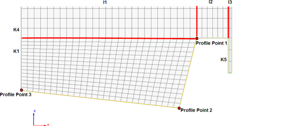
Once you have a profile, the first step in the mesh workflow is to specify the desired mesh topology that is appropriate for the imported piston-bowl shape. For this simple flat-piston-bowl geometry, Topology 3 will be used since it is a square-shaped bowl, as shown in Figure 2.2: Template for Topology #3 . For this topology there are only 3 coordinates needed to define the profile and exactly 3 are required.
Go to the Mesh Parameters node in the SMG tree. Select Topology 3 in the Topology drop-down menu. If you would like to see the topology template selected, click the Show Topology button. It should look like the figure shown in Figure 2.2: Template for Topology #3 .
Next, enter the cell counts between the different control points, as indicated in the Topology 3 diagram, and in the schematic drawing in the 3-D display window. The parameters we will enter are as follows:
Circumferential Cell Count = 21
Radial Cell Count 1 (i1) = 16
Radial Cell Count 2 (i2) = 11
Radial Cell Count 3 (i3) = 3
Axial Cell Count 1 (k1) = 11
Axial Cell Count 4 (k4) = 21
Axial Cell Count 5 (k5) = 11
Smoothing Passes = 20 (default value; works well for most cases)
Once all the settings are specified, click Apply. Review the outline of the profile information in the 3-D View panel to verify that the settings make sense.
Then use the Generate a Mesh
 icon at the top of the Mesh Parameters Editor panel in the Sector Mesh
Generator. Ansys Forte will automatically generate the sector mesh. When it is finished, the
resulting mesh will appear for your review in the 3-D View window within the Sector Mesh
Generator window, as shown in Figure 2.3: Diesel sector sample mesh as generated in the Sector Mesh Generator.
. (You may need to click the
Refit
icon at the top of the Mesh Parameters Editor panel in the Sector Mesh
Generator. Ansys Forte will automatically generate the sector mesh. When it is finished, the
resulting mesh will appear for your review in the 3-D View window within the Sector Mesh
Generator window, as shown in Figure 2.3: Diesel sector sample mesh as generated in the Sector Mesh Generator.
. (You may need to click the
Refit  icon.)
Note: You can modify settings here to refine or coarsen the mesh, for example, and re-generate, or you can open (import) the newly created mesh into the sample project into Ansys Forte. Alternatively, you can use the Save to File button to export to a mesh file that can later be imported into Ansys Forte.
For this tutorial, click Mesh Parameters in the Sector Mesh Generator's Project tree, then click the Import to Forte Project
 icon in the Editor panel. Now go to the Simulate window and see the new
Geometry items added to the Workflow tree. If you cannot see the mesh that you just generated
displayed in the main 3-D View panel, right-click these Geometry items for options to make
their Mesh visible. To center and resize the mesh display, click the
Refit icon on the View toolbar.
icon in the Editor panel. Now go to the Simulate window and see the new
Geometry items added to the Workflow tree. If you cannot see the mesh that you just generated
displayed in the main 3-D View panel, right-click these Geometry items for options to make
their Mesh visible. To center and resize the mesh display, click the
Refit icon on the View toolbar.If the Sector Mesh Generator window is still open, you can close it.
Now that the mesh has been defined, you can set up the models and solver options using the guided tasks in the Ansys Forte Simulate Workflow tree. In many cases, default parameters are assumed and employed, such that no input is required. The required inputs and changes to the setup panels for this case are described here.
In the Workflow tree, expand Models. In the following steps you will turn ON (check-mark) several models and configure parameters for them in their Editor panels.
Note: You can change the display properties of items in the 3-D View by selecting the items in the Workflow tree and right-clicking then selecting options from the context menu, such as turning their visibility ON/OFF, display of the mesh, or level of opacity.
Models > Chemistry/Materials: In the Workflow tree, under Models, select Chemistry/Materials. On the Chemistry/Materials icon bar, click the Import Chemistry
 icon. This opens a file browser where you can navigate to and select a
chemistry set file. For this project, however, we use a pre-installed chemistry set that comes
with Ansys Forte. This is a simplified, reduced n-heptane mechanism that can be used to represent
the diesel fuel under conventional diesel-engine combustion conditions. To load this file,
browse to the System Data directory, which can be
accessed from this file browser by clicking the data radio button in the
upper right-hand sub-panel of the browser window, and locate the pre-installed
Diesel_1comp_35sp.cks file. The chemistry file is a standard
Ansys Chemkin chemistry-set file. More information about the chemistry set and the files referenced
within it can be found in the Forte User's Guide.
icon. This opens a file browser where you can navigate to and select a
chemistry set file. For this project, however, we use a pre-installed chemistry set that comes
with Ansys Forte. This is a simplified, reduced n-heptane mechanism that can be used to represent
the diesel fuel under conventional diesel-engine combustion conditions. To load this file,
browse to the System Data directory, which can be
accessed from this file browser by clicking the data radio button in the
upper right-hand sub-panel of the browser window, and locate the pre-installed
Diesel_1comp_35sp.cks file. The chemistry file is a standard
Ansys Chemkin chemistry-set file. More information about the chemistry set and the files referenced
within it can be found in the Forte User's Guide.Note: You can respond Yes or No to the "View chemistry set information?" prompt. A Yes response displays the chemistry set file in a viewer.
Models > Transport: For this node, keep all the default settings.
Models > Spray Model: Since this is a direct-injection case, turn ON (check) Spray Model to display its icon bar (action bar) in the Editor panel.
For the basic Spray Properties, select Radius of Influence Model for the Droplet Collision Model and set 0.2 cm as the Radius of Influence. The Use Vaporization Model option should be ON (checked, its default value). Click Apply.
Create Injector: The icon bar provides two spray-injector options: Hollow Cone or Solid Cone. For the diesel injector, click the Solid Cone
 icon. In the dialog that opens, name the Spray Model as
"Injector 1". This opens another icon bar and Editor panel
for the new solid-cone spray model. In the Editor panel, configure the model parameters for
the solid-cone spray model.
icon. In the dialog that opens, name the Spray Model as
"Injector 1". This opens another icon bar and Editor panel
for the new solid-cone spray model. In the Editor panel, configure the model parameters for
the solid-cone spray model. Composition: Select Create New... in the Composition drop-down menu under Settings and click the Pencil
icon to open the Fuel Mixture Editor. In the Fuel Mixture panel,
click the Add Species button and select nc7h16
(that is, n-heptane) as the Species,
n-Tetradecane as the Physical Properties and
1.0 as the Mass Fraction. (Note that you must
press ENTER after entering the values in the table.) At the bottom of the panel, type a name such as "n-heptane". Click Save and Close the window.
Under the Injection Type, select Pulsed Injection and change the Parcel Specification to Number Of Parcels and set Injected Parcel Count = 30,000.
Set Inflow Droplet Temperature = 368.0 K.
Set Spray Initialization to Discharge Coefficient and Angle, and Discharge Coefficient = 0.7, and Cone Angle = –15.0 degrees.
Keep default values for Droplet Size Distribution and, under the Solid Cone Breakup Model Settings, the KH Model Constants, RT Model Constants, and Use Gas-Jet Model.
Click Apply.
Create a Nozzle: Click the New Nozzle
 icon on the Spray icon bar and name the nozzle "Nozzle
1". Nozzle 1 then appears in the Workflow tree, and the Editor panel and
icon bar transform to allow specification of the Nozzle geometry and orientation. In the
Editor panel, set the Reference Frame parameters to specify the nozzle location and
direction. Keep the default Global Origin and use the following
settings:
icon on the Spray icon bar and name the nozzle "Nozzle
1". Nozzle 1 then appears in the Workflow tree, and the Editor panel and
icon bar transform to allow specification of the Nozzle geometry and orientation. In the
Editor panel, set the Reference Frame parameters to specify the nozzle location and
direction. Keep the default Global Origin and use the following
settings:Location > Coord. System = Cylindrical, with R = 0.15 cm, θ = 22.5 degrees, and A = 19.368 cm.
Spray Direction > Coord. System = Spherical, θ = 104.0 degrees, and ϕ = 22.5 degrees.
Nozzle Size > Area = 0.000302 cm2.
Click Apply. You can see the nozzle appear at the top of the geometry. (You may wish to make the Geometry less opaque by right-clicking the Geometry item and selecting a lower value for Opacity, or change the color of the nozzle itself, to make the nozzle easier to see in the interior.)
Create an Injection: In the Workflow tree, click Injector 1 again and click the New Injection
 icon on the Injector 1 icon bar and name the
injection Injection 1. The new Injection item appears in the Workflow
tree, and the Editor panel and the icon bar transform to allow specification of the
injection properties. In the Editor panel, keep the Pulsed Injection
Type (default), select Crank Angle as the Timing
Option and then specify the Start of injection and
Duration of injection as –22.5 and
7.75 degrees ATDC, respectively. Set the Total Injected
Mass = 0.0535 g. Click Apply.
icon on the Injector 1 icon bar and name the
injection Injection 1. The new Injection item appears in the Workflow
tree, and the Editor panel and the icon bar transform to allow specification of the
injection properties. In the Editor panel, keep the Pulsed Injection
Type (default), select Crank Angle as the Timing
Option and then specify the Start of injection and
Duration of injection as –22.5 and
7.75 degrees ATDC, respectively. Set the Total Injected
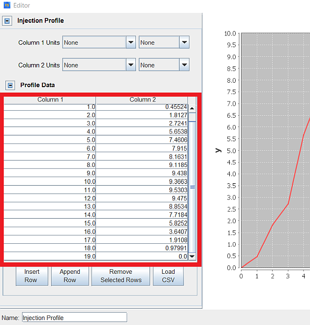
Mass = 0.0535 g. Click Apply. Injection Profile: Select Create new... in the profile drop-down menu next to Velocity Profile, then click the Pencil
icon to open a new window with the Profile Editor. The new Injection
Profile item appears in the Workflow tree; also the Editor panel and the icon bar transform
to the new Injection Profile. In the Profile Editor window, make sure all the
Units are set to None for both columns (the
dimensionless data is automatically scaled within Ansys Forte to match the mass and duration of
injection) and click the Load CSV button at the bottom of the panel
(you may have to expand the panel size to see the button). Navigate to the
InjectionProfile.csv file (see Data Provided
). Select
Comma as the Column delimiter and turn ON
Read Column Titles and load the profile file. Alternatively, you can
type in the Injection Profile data in the table on the Editor panel or copy and paste from a
spreadsheet or 3rd-party editor. Go to Profile Name at the bottom-left
of the panel and name the new profile Injection Profile. Once the data
is entered, click Save and Close the Profile
Editor window and then click Apply in the Ansys Forte Editor panel.
Models > Soot Model: Turn ON the Soot Model. This creates the Settings item. In the Editor panel, accept all the defaults.
Under Boundary Conditions in the Workflow tree, specify the Boundary conditions in the Editor panels associated with each of the four boundary conditions created by importing the mesh. By default the Wall Slip Condition for all of the wall boundaries will be set to Law of the Wall. Leave this default setting as well as the default check box that turns ON heat transfer to the wall.
Boundary Conditions > Piston: Set Wall Temperature = 500.0 K. Turn ON Wall Motion with Motion Type set to Slider Crank. The other parameters should be:
Stroke = 15.24 cm
Connecting Rod Length = 30.48 cm
Bore = 13.97 cm (pre-determined by the Sector Mesh Generator)
Accept the defaults of Piston is Offset = unchecked (OFF).
For Reference Frame, accept the default Global Origin and Direction parameters.
Click Apply.
Boundary Conditions > Periodicity: Set the Sector Angle = 45 degrees, and multi-select both Periodic A and Periodic B boundaries on which to apply this boundary condition. Click Apply.
Boundary Conditions > Head: Set Wall Temperature = 470.0 K. Click Apply.
Boundary Conditions > Liner: Set Wall Temperature = 420.0 K. Click Apply.
Initial Conditions > Region 1 Initialization (Main): Specify the parameters for the initial conditions as follows:
Composition: Select Constant and then Create new gas mixture... in the Composition drop-down menu and click the Pencil
icon and to launch the Composition Editor. Set these parameters: set the
Composition = Mole Fraction (not the default
Mass Fraction). Then click the Add Species button
and select both o2 and n2 to add. When both
o2 and n2 are in the Species column in the
Composition table, enter 0.126 for the o2
Fraction and 0.874 for n2. Name this
"Composition 1" in the text field at the bottom of the Gas Mixture window. Click
Save and close the Composition Editor.Temperature = 362.0 K
Pressure = 2.215 bar (Note: This is not the default unit.)
Turbulence: Select Constant, and then in the drop-down menu for the initial Turbulence parameters, select Turbulent Kinetic Energy and Length Scale as the way in which we will specify the initial turbulence. For this option we provide an explicit value for the initial turbulent kinetic energy, but use a length-scale approximation to determine the turbulence dissipation energy. Use the following values:
Turbulent Kinetic Energy = 10,000cm2/sec2
Turbulent Length Scale = 1.0 cm
Velocity: Select Engine Swirl in the Velocity drop-down and then specify the swirl profile parameters:
Initial Swirl Ratio = 0.5
Initial Swirl Profile Factor = 3.11
Initialize Velocity Components Normal to Piston = ON
Note: If you want to estimate the turbulent kinetic energy (TKE) as a fraction of the piston speed, let the fraction be F and stroke is ms-1, the value you would enter then would be

Piston Boundary: Select Piston from the selection list.
Click Apply in the Region 1 Initialization Editor panel.
In the Silulation Controls panel, under Simulation Limits, select Crank Angle Based in the Simulation End Points drop-down menu and specify the following parameters:
Initial Crank Angle = -165.0
Final Simulation Crank Angle = 125.0 degrees. (These two angles correspond to Intake Valve Open and Exhaust Valve Closing, respectively).
RPM = 1,200.0
Cycle Type is 4-Stroke.
Click Apply.
Simulation Controls > Time Step: For the Advanced Time Step Control Options, specify:
Rate of Strain Factor = 0.6
Convection Factor = 0.2
Click Apply.
Simulation Controls > Chemistry Solver:
Turn ON (check) Use Dynamic Cell Clustering and accept its defaults.
At the bottom of the panel, set Activate Chemistry to Conditionally, specifying When Temperature is Reached, setting Threshold Temperature = 600.0 K. Click Apply.
Output Controls > Spatially Resolved:
For the Output Timing Control option, select the Crank Angle option.
Turn ON (check) Interval Based Crank Angle Outputs.
Output every = 5.0 degrees.
Turn ON (check) User Defined Crank Angle Outputs and select Create new... in the drop-down menu to open the Profile Editor. Import the UserCrankAngleOutputs.csv table of data that contains crank angles going from -22 to +20, with increment 1, units of Angle and Degree, and file named UserCrankAngleOutputs. This assures that we get more resolved outputs around the spray, without requiring the same resolution throughout the simulation.
For Spatially Resolved Species, move these species to the Selection list: nc7h16, o2, n2, co2, h2o, co, no, and no2. Click Apply.
Output Controls > Spatially Averaged And Spray:
For the Spatially Averaged Output Control, select the Crank Angle option and specify Output Every = 1.0 degree.
For Spatially Averaged Species, select all and move all species to the Selection list. Click Apply.
Output Controls > Restart Data: In the Workflow tree, check the box for Restart Data and then in the Restart panel, turn ON (check) Write Restart File at Last Simulation Step. Turn OFF (uncheck) any other boxes on the panel. Click Apply.
In the Workflow tree, under Run Simulation, select Nominal to open the run control interface.
Click the blue arrow Submit Run button to start running the case. The Status changes to "Running."
To interrupt the run, click the Stop Run button. Then the Status becomes "Stopped".
To start over or restart, click Submit Run again.
The progress of the simulation can be monitored during a run. To monitor the averaged value of simulation variables, click the Monitor Runs
 icon on the Run Simulation icon bar.
A new window then appears, with a list of variables that can be plotted on the left panel in the window (as described in the Forte User's Guide). To select one or more variables to plot, check the boxes in front of them in the Monitor Data panel.
While the simulation jobs are running, they are writing results into the solution file (.ftind and .ftres) and also writing to several .csv files that can be used for plotting intermediate results. Learn more about monitoring runs in the Forte User's Guide.
You can save the project at this point using the File > Save command. Rename the project to avoid overwriting the original .ftsim file.
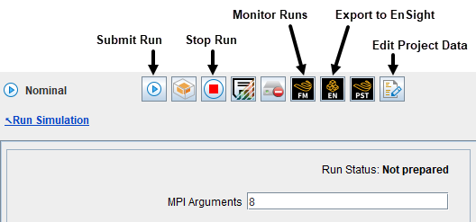
When a run is finished, the Status becomes Complete in the Run panel of the main Simulate User Interface window. In the Editor panel, click the EnSight button to export to that application.
This case models the engine experiment from the following paper:
Singh, S., Reitz, R. D., and Musculus, M. P. B. Comparison of the characteristic time (CTC), representative interactive flamelet (RIF), and direct integration with detailed chemistry models against optical diagnostic data for multi-mode combustion in a heavy-duty DI diesel engine. SAE paper 2006-01-0055, 2006.