This tutorial describes the Conjugate Heat Transfer (CHT) simulation of a generic diesel engine case. When measurement data are not available, it is hard to set the wall temperatures in a typical stand-alone CFD simulation. For this reason, coupling thermal analysis in the solid walls with the CFD simulation can help the accuracy in the setup. The thermal analysis receives heat transfer data from the CFD simulation and predicts wall temperatures, those are then sent back to the CFD simulation to correct the boundary conditions. This coupled simulation continues, until the thermal data transferred between the CFD and the thermal analysis converges. The exchange of data is a seamless workflow managed by System Coupling (see System Coupling User's Guide), which is a general-purpose tool to couple solutions from different Ansys solvers. The in-cylinder flow and combustion are solved by Ansys Forte, while the thermal analysis and the coolant flow are performed by Ansys Fluent. The CHT simulation is carried out by an iterative coupling loop with an alternate execution of the two solvers, and the exchange of heat-transfer-related data at common interfaces.
The files for this tutorial are obtained by downloading the
syc_generic_engine.zip file
here
.
Note: Forte tutorial files are also available as a bundled downloadable package. To access the files on the Ansys Help site, go to the Forte page at: ansyshelp.ansys.com.
You have the opportunity to select the location for the files when you download and uncompress the sample files. Once downloaded and unpacked, they include:
run.py- System Coupling python script that defines the coupling of Fluent to Forte, the coupling interfaces, the data being transferred, the stopping criteria of the iteration, and is used to start the coupled simulation.fluent.scp- Fluent XML System Coupling file that defines the fluent input and output variables.In the
fortedirectory:DieselEngine.ftsim- the Forte project file, which simulates the full-cycle, in-cylinder combustion process.
In the
fluentdirectory:EngineBlock.cas.h5- the Fluent project file, which simulates the coolant flow and the thermal analysis of the surrounding engine block.
Note: When running this example, ensure the file structure is consistent with
run.py and fluent.scp in the local folder where you
are going to run the tutorial, and that there are two sub-folders,
forte and fluent, with the corresponding project files
in each sub-directory.
Note: This tutorial is based on a fully configured sample project that contains the tutorial project settings. The description provided here covers the key points of the project set-up but is not intended to explain every parameter setting in the project. The project files have all custom and default parameters already configured; the text highlights only the significant points of the tutorial.
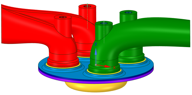
To establish a CHT simulation, the System Coupling participants must be set up first. A participant is an individual simulation that acts as component of the coupled simulation and in this tutorial they are ANSYS Forte and Ansys Fluent. Each participant has its own physical domain (see Figure 25.1: Forte simulation domain and Figure 25.2: Fluent simulation domain), and its own set of boundary conditions. The two participants exchange data at the head and liner of the cylinder; the combustion simulation in Forte provides heat transfer rate data to be used as boundary conditions in the flow and thermal conduction analysis in Fluent, which in turn predicts temperature distributions to update Forte's boundary conditions. The iterative loop continues, and the simulation stops when the data transferred at both the interfaces converge.
The CHT simulation is already set up in the downloaded files of this tutorial. You can directly run the simulation (see the instructions in Launching the CHT Simulation) using these files. The instructions provided in this section are an overview of the project settings.
Before setting and launching the simulation it is important to have the right folder structure in your own working directory. With this intent, follow these guidelines:
Create a working directory.
Copy the downloaded System Coupling script file (
run.py) and the Fluent XML System Coupling file (fluent.scp) into the working directory.Copy the downloaded sub-folders (
forte, fluent) into the working directory as well.
As mentioned, from the System Coupling point of view, we have two participants:
First is Forte with:
input variable Temperature
output variable Heat Rate
Second is Fluent with:
input variable Heat Rate
output variable Temperature
This tutorial simulates the full cycle of a generic 4-stroke diesel engine. Most of the project settings are similar to those of a stand-alone Forte simulation for IC engines. The chemistry set used is the Diesel_1comp_35sp.cks, the turbulence model is the RNG k-ε model, and the mesh refinements follow the Forte Best Practices. The engine specifications are listed in Table 25.1: Engine specification.
Table 25.1: Engine specification
| Compression ratio | 13.75 |
| Bore | 9 cm |
| Stroke | 8 cm |
| RPM | 1500 |
| Start of fuel injection | 710 CA |
| Duration of injection | 30 CA |
| Injected fuel amount | 65 mg |
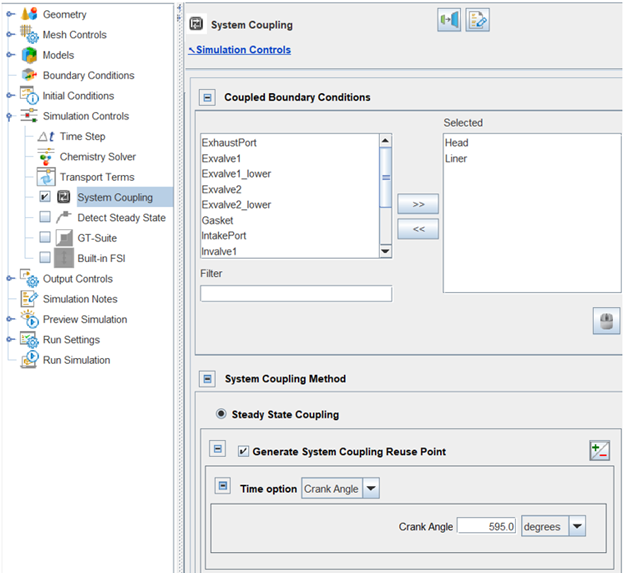
At a distance of 1 mm below the head, there are 6 nozzles injecting 100% n-heptane, inclined by 120 degrees with respect to the vertical axis, using all the default values for the spray modeling settings. In the initial conditions panel, the intake region is initialized with 350 K and 2 bar while the exhaust region with 1000 K and 3 bar. The boundary conditions of interest for the system coupling simulation are tentatively set to 550 K and 470 K for the head and the liner respectively; they will be updated by Fluent via system coupling during the following iterations. To allow so, and send back updated heat rate data to Fluent, the System Coupling check box in the Simulation Controls node of the Workflow tree must be activated as in Figure 25.3: Enable the System Coupling node, and the Head and Liner surfaces must be selected. Forte will then automatically create two extra .csv files called wall_sampling_Head_system_coupling.csv and wall_sampling_Liner_system_coupling.csv to store time-averaged heat rate data on the head and liner boundaries automatically transferred to Fluent. Navigating through the System Coupling node, the Steady State Coupling option is selected since the Fluent counterpart of this simulation is set to be pseudo-transient. It can be noticed that the Generate System Coupling Reuse Point option is also selected, associated to a crank angle of 595 degrees. This means that during the first iteration, Forte generates a restart point at 595 CA, and all the following iterations will reuse the previously solved gas exchange portion (132 to 595 CA), reducing the turn-around time. Finally, the Heat Rate needs to be selected in the Output Variables panel.
Note: The heat transfer rate data are defined on the surface mesh elements of the wall surface requested for System Coupling. Therefore, it is good practice to ensure that the surface mesh has sufficient spatial resolution so that the heat transfer rate output at the interface also has the same spatial resolution. To check the surface mesh resolution, go to Geometry in the Workflow tree and select the surface patch that corresponds to the Head boundary condition. In this case, the surface patch is named cyl-head. Right-click the surface patch and check the Mesh option to visualize the surface mesh in the 3-D View. Do the same with the surface patch named liner.
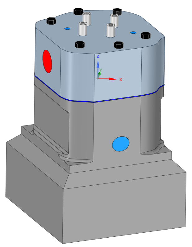
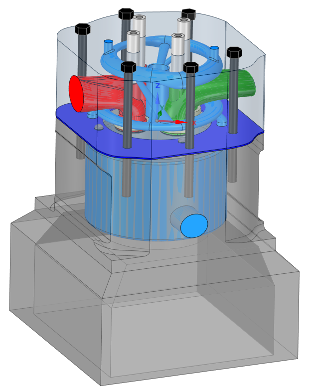
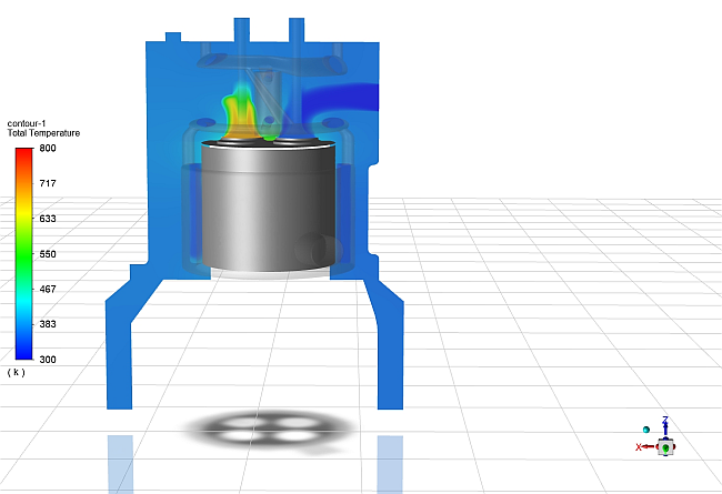
The coolant flow and thermal analysis of the generic diesel engine is performed in Fluent. The geometry is representative of a realistic engine with a single cylinder. When opening the EngineBlock.cas.h5 project file with the Fluent user interface, take a moment to explore the full domain and identify the different components. In Figure 25.4: Inside of the Fluent domain, one can see 6 bolts colored in black, valves and valve guides in gray, the gasket in dark blue, the light blue fluid region, which is the coolant jacket surrounding the cylinder engine, and finally the red and green components are both fluid regions, respectively the exhaust and the intake port of the engine. Each body has its own material property set.
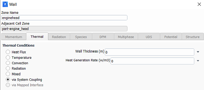
As previously mentioned, the setup is a pseudo-transient simulation solving the flow and the energy equation. The turbulence model in use is the SST-k-omega. In a similar fashion to the Forte setup, the coupled boundaries enginehead and liner must be set as via System Coupling, as shown in Figure 25.5: Setting up Fluent coupled boundaries.
Normally, after the Fluent project is set up, you must export the project
settings for System Coupling's use. To do this, navigate to File > Export >
System Coupling > Write SCP File, and save the project settings to an
.scp file. In this tutorial, you do not need this step, because the
project settings have been saved to fluent.scp and placed in the run
directory. For more information about how to prepare a Fluent project for
System Coupling, refer to the Fluent User's Guide, "Performing Command Line System
Coupling."
The System Coupling setup is defined in the python script file named run.py. It invokes several functions, including loading the participants' project information, setting up the coupling interface, specifying both the control for coupled iterations and the options to promote convergence, and launching the simulation. The python script used in this tutorial is shown below as an example. You may use it as a template when setting up a new coupled simulation.
Example 25.1: run.py python script
import os

# Add Forte as coupling participant
forte = AddParticipant(InputFile = os.path.join('forte', 'DieselEngine.ftsim'))

# Add Fluent as coupling participant
fluent = AddParticipant(InputFile = ('fluent.scp'))


# Define coupling interfaces and data transfers
iName_1 = AddInterface(SideOneParticipant = fluent,
                       SideOneRegions = ['enginehead'],
                       SideTwoParticipant = forte,
                       SideTwoRegions = ['Head'])

iheatrate_1 = AddDataTransfer(Interface = iName_1,
                              TargetSide = 'One',
                              SideOneVariable = 'heatflow',
                              SideTwoVariable = 'HEATR')

itemperature_1 = AddDataTransfer(Interface = iName_1,
                                 TargetSide = 'Two',
                                 SideOneVariable = 'temperature',
                                 SideTwoVariable = 'TEMP')

iName_2 = AddInterface(SideOneParticipant = fluent,
                        SideOneRegions = ['liner'],
                        SideTwoParticipant = forte,
                        SideTwoRegions = ['Liner'])

iheatrate_2 = AddDataTransfer(Interface = iName_2,
                               TargetSide = 'One',
                               SideOneVariable = 'heatflow',
                               SideTwoVariable = 'HEATR')

itemperature_2 = AddDataTransfer(Interface = iName_2,
                                  TargetSide = 'Two',
                                  SideOneVariable = 'temperature',
                                  SideTwoVariable = 'TEMP')

dm = DatamodelRoot()
# Set maximum and minimum iterations and use ramping and relaxation to stablise convergence
dm.SolutionControl.MaximumIterations= 40
dm.SolutionControl.MinimumIterations= 1
dm.AnalysisControl.GlobalStabilization.Option='Quasi-Newton'
dm.AnalysisControl.GlobalStabilization.InitialRelaxationFactor=1
dm.CouplingInterface[iName_1].DataTransfer[iheatrate_1].Stabilization.Option = 'Quasi-Newton'
dm.CouplingInterface[iName_1].DataTransfer[iheatrate_1].Stabilization.InitialRelaxationFactor = 1
dm.CouplingInterface[iName_1].DataTransfer[iheatrate_1].ConvergenceTarget = 0.5

dm.CouplingInterface[iName_2].DataTransfer[iheatrate_2].Stabilization.Option = 'Quasi-Newton'
dm.CouplingInterface[iName_2].DataTransfer[iheatrate_2].Stabilization.InitialRelaxationFactor = 1
dm.CouplingInterface[iName_2].DataTransfer[iheatrate_2].ConvergenceTarget = 0.5


dm.ActivateHidden.BetaFeatures = True
dm.OutputControl.GenerateCSVChartOutput = True
dm.OutputControl.Option = 'EveryIteration'

# Launch the coupled simulation
Solve()
The order in which the participants are started is given by the order in which they are listed in the run.py script, whereas it is completely unimportant the order in which the interfaces are listed. The first interface identifies the Fluent enginehead patch coupled with the Forte boundary Head (note that these names are case-sensitive) while the second interface refers to the Fluent patch liner coupled with the Forte boundary Liner. We are transferring Forte Heat Rate (HEATR) to Fluent's heatflow and Fluent's temperatures to Forte's boundary conditions (TEMP). Before starting the simulation it is important to choose the appropriate coupling controls. In this tutorial the best practice makes use of the Quasi-Newton solution stabilization and acceleration method to transfer Heat Rate data from Forte to Fluent with no initial relaxation factor (see "System Coupling Data Transfers" in the System Coupling User's Guide). The convergence targets for temperature data transfer are kept as the default, 0.01, while the ones for heat rate are loosened up to 0.5 for both coupled surfaces. For post-processing purposes an Ansys EnSight output is generated at each run (EveryIteration), and the option for Generate CSV Chart Output has been activated.
To run System Coupling, you must run the System Coupling python environment and pass the
run.py script.
On Windows, open a CMD prompt and type:
call "c:\Program Files\ANSYS Inc\v242\SystemCoupling\bin\systemcoupling" -t8 -R run.py
On Linux at the command prompt, type:
sh $home/ansys_inc/v242/SystemCoupling/bin/systemcoupling -t8 -R run.py
Note: Here 8 is just an example of how to select the number of cores to use. For this tutorial we have used 126 cores. Additionally, if you changed the location of your ANSYS install, do not forget to change the path to v242 appropriately.
The System Coupling iterations will run until convergence is accomplished as defined in the python script. The coupled simulation converges in 4 iterations under the current settings.
Once the coupled simulation has converged, you can examine the Forte and Fluent
simulation results in their directories. In the forte directory, you will
see a list of folders named as SCRun_<number>, where <number>
is the iteration number of the coupled simulation.
Figure 25.6: Averaged heat transfer flux on the engine cylinder liner
as a function of crank angle in Forte shows a zoom-in of the spatially averaged
wall heat transfer fluxes as a function of crank angle for both the head and the liner.
Especially noticeable at the head is the effect of the wall temperature boundary
conditions being updated, while in
Figure 25.9: Temperature contour on a zx-plane at y= -0.018 m OUTSIDE the engine
cylinder and
Figure 25.10: Temperature contour on a zx-plane at y= -0.018 m INSIDE the engine
cylinder the overall solution expressed in terms
of spatially averaged Pressure, Apparent Heat Release Rate, and Temperature is
insensitive to Temperature stratification.
Figure 25.6: Averaged heat transfer flux on the engine cylinder liner as a function of crank angle in Forte
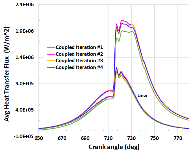
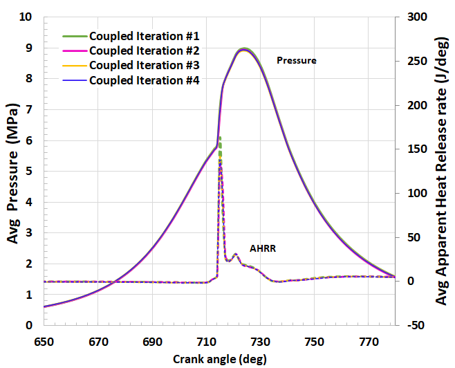
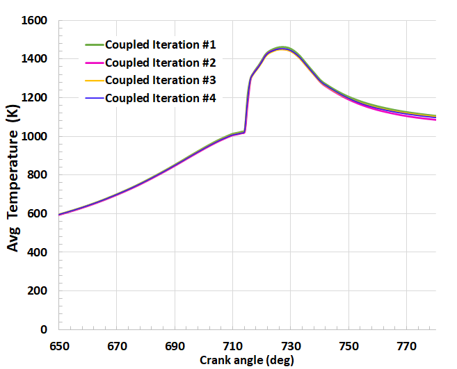
Figure 25.9: Temperature contour on a zx-plane at y= -0.018 m OUTSIDE the engine cylinder shows the spatially resolved temperature outside the cylinder engine (Fluent domain) on a cut plane at y =-0.018 m. In dark gray you can identify the two coupled interfaces, head and liner, while in light gray the exhaust valve 1, the intake valve 1 and the coolant jacket are displayed to facilitate the understanding of the geometry orientation. The figure has been realized by loading the *.dat results stored in the fluent folder at the end of the coupled simulation.
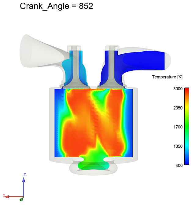
On the same cut plane at y=-0.018 m, Figure 25.10: Temperature contour on a zx-plane at y= -0.018 m INSIDE the engine cylinder shows the instantaneous temperature distribution inside the cylinder engine (Forte domain) at 852 CA of the converged iteration.
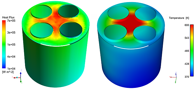
Finally, Figure 25.11: Heat flux and temperature distribution averaged in time on the head and liner shows the spatially resolved and time averaged variables on the two coupled interfaces where the data transfer occurs. Notice the small gap between the head and the liner in both domains that represent the gasket, the surface is not coupled and therefore not reported in this figure.
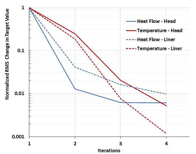
It is also possible to monitor and analyze the convergence status of the simulation by turning on the CSV Chart Output feature in the run.py as follows
DatamodelRoot().OutputControl.GenerateCSVChartOutput = True
This will create an Interface-<i>.csv file per
each coupled boundary in the SyC directory from which the
normalized RMS change of data transferred can be extracted, as shown in
Figure 25.12: Normalized RMS
Change in Target Value.Note that the y-axis is expressed in a
logarithmic scale.