Conjugate Heat Transfer (CHT) is a useful procedure in CFD because it provides realistic thermal boundary conditions. Most CFD simulations of heat transfer problems apply assumed wall temperatures as boundary conditions, without any available measured data. Such assumption can affect the validity and usefulness of the CFD simulation results. CHT has addressed this challenge by coupling the simulations of the fluid and solid on the each side of the wall boundary, and obtaining the wall temperature in a predictive manner.
In this tutorial, we consider a CHT simulation in an internal combustion engine application. The in-cylinder flow and combustion processes are simulated by a transient CFD analysis using Ansys Forte and is coupled with a steady-state thermal analysis of the engine block using Ansys Fluent. The coupled simulation starts with an assumed wall temperature for the in-cylinder CFD simulation, with which the heat transfer rate through the cylinder wall is computed. Subsequently, the thermal analysis of the engine block is performed by using the heat transfer rate as a boundary condition. It computes the wall temperature and uses it to update the boundary condition for the in-cylinder combustion CFD for the second iteration of a coupled simulation. In each of these iterations, transfer of the data for heat transfer rate and wall temperature between the two simulations is handled automatically by Ansys System Coupling (see System Coupling User's Guide), without the need of user intervention. The coupled simulation continues iteration by iteration, until the differences between consecutive data transfers meet the set criteria for convergence, or the maximum number of iterations is reached. After the CHT simulation converges, a more realistic wall temperature distribution on the coupled wall surface is obtained.
The files for this tutorial are obtained by downloading the
system_coupling_engine.zip file
here
.
Note: Forte tutorial files are also available as a bundled downloadable package. To access the files on the Ansys Help site, go to the Forte page at: ansyshelp.ansys.com.
You have the opportunity to select the location for the files when you download and uncompress the sample files. Once downloaded and unpacked, they include:
run.py- System Coupling python script that defines the coupling of Fluent to Forte, the coupling interfaces, the data being transferred, the stopping criteria of the iteration, and is used to start the coupled simulation.fluent.scp- Fluent XML System Coupling file that defines the fluent input and output variables.In the
fortedirectory:Engine.ftsim- the Forte project file, which simulates the in-cylinder combustion process.
In the
fluentdirectory:Metal_block.cas- the Fluent case file, which simulates the thermal analysis of the cylinder wall.
Note: When running this example, ensure the file structure is consistent with
run.py and fluent.scp in the local folder where
you are going to run the tutorial, and that there are two sub-folders,
forte and fluent, with the corresponding project
files in each sub-directory.
Note: This tutorial is based on a fully configured sample project that contains the tutorial project settings. The description provided here covers the key points of the project set-up but is not intended to explain every parameter setting in the project. The project files have all custom and default parameters already configured; the text highlights only the significant points of the tutorial.
The CHT simulation setup is provided in the downloaded files provided with this tutorial. You can directly run the simulation (see instructions in Launching the CHT Simulation) using these files. In this section, we provide an overview of the project settings that are specific to this tutorial but also helpful for setting up a coupled simulation in general. To establish a CHT simulation, the System Coupling participants are set up first with proper boundary conditions. They are the individual simulations that act as components of the coupled simulation. The interfaces that allow data transfer between the participants are defined as System Coupling boundary conditions.
In this tutorial, there are two participants:
In-cylinder flow and combustion processes of the IC engine analyzed with Ansys Forte;
Thermal analysis of the engine block analyzed with Ansys Fluent.
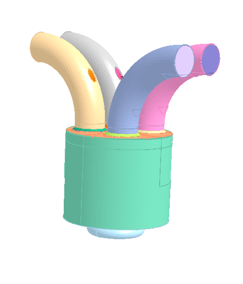
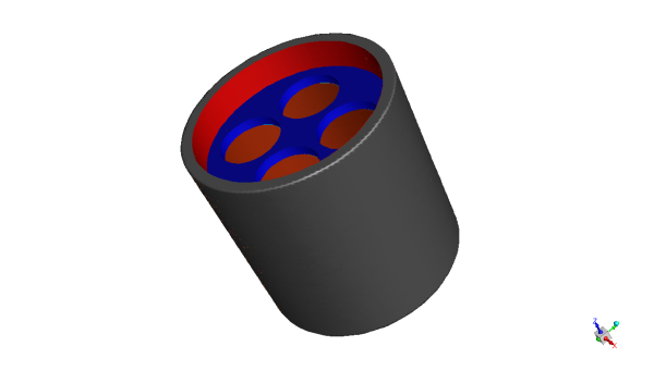
The simulation domains of the two participants are shown in Figure 24.1: Simulation domain in Forte of flow and combustion analysis and Figure 24.2: Simulation domain in Fluent for the cylinder wall's thermal analysis, respectively.
In this tutorial, the aim of the CHT simulation is to determine a realistic temperature distribution on the engine cylinder head and liner, which serve as the coupling interfaces. Therefore, the Forte simulation transfers the computed wall heat transfer through the cylinder head and liner to the Fluent simulation, while the Fluent simulation transfers the computed wall temperature data on the same surfaces back to the Forte simulation.
Both the participants and the System Coupling have been set up for this tutorial in the downloaded files. For the remaining parts of this section, we will review the setup procedure for the coupling participants (Forte and Fluent) and the Ansys System Coupling settings.
Create a working directory. For example:
C:\users\Download\CHT.Copy the downloaded System Coupling script file (
run.py) and the Fluent XML System Coupling file (fluent.scp) into the working directory.Copy the downloaded sub-folders (
forte, fluent) into the working directory.
As mentioned, from the System Coupling point of view we have two participants:
First is Forte with:
input variable Temperature
output variable Heat Rate
Second is Fluent with:
input variable Heat Rate
output variable Temperature
A generic 4-stroke diesel engine is considered in this tutorial, and its specifications are listed in Table 24.1: Engine specification in Forte Setup.
Table 24.1: Engine specification in Forte Setup
| Compression ratio | 17.3 |
| Engine bore size | 9.0 cm |
| Start of fuel injection | 710 crank angle degrees |
| Injected fuel amount | 0.25 g |
| Intake-Valve-Closure | 580 crank angle degrees |
| IVC temperature | 350 K |
You can load the Forte project file (Engine.ftsim) into the
Forte
Simulate user interface to review its settings. The
simulation domain used in Forte is shown in Figure 24.1: Simulation domain in Forte of flow and combustion analysis. It includes the combustion
chamber of a single cylinder as well as the intake and exhaust ports connected to
it. For simplicity, the intake and exhaust valves are assumed to be closed during
the simulation, which runs from the Intake-Valve-Closure timing to the
Exhaust-Valve-Opening timing. Diesel fuel injection occurs at 10 degrees before the
piston reaches its Top-Dead-Center.
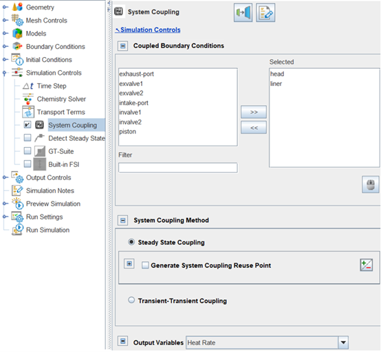
Most of the project settings are similar to those of a stand-alone Forte simulation for IC engines. To perform a System Coupling simulation, go to the Simulation Controls node, check (turn ON) the System Coupling box and be sure to select boundary conditions associated with the coupled interfaces head and liner. Select Heat Rate as the Output variable, and select the Steady State Coupling method, as shown as in Figure 24.3: Enable System Coupling for the cylinder head and liner boundary conditions in Forte. Note that a uniform and fixed wall temperature of 400 K is specified for head and 600 K has been set for liner as an initial guess to start the coupled simulation. The wall temperature will be updated by the data transferred from Fluent in the subsequent iterations.
During the coupled simulation, Forte will automatically create two extra .csv files called wall_sampling_head_system_coupling.csv and wall_sampling_liner_system_coupling.csv to store time-averaged heat transfer rate data on the head and liner boundaries. These files are in the Forte run folder and will be used by System Coupling automatically during the coupled simulation.
Note: The heat transfer rate data are defined on the surface mesh elements of the wall surface requested for System Coupling. Therefore, it is good practice to ensure that the surface mesh has sufficient spatial resolution, so that the heat transfer rate output at the interface has the same spatial resolution as well. To check the surface mesh resolution, go to Geometry and select the surface patch that corresponds to the head boundary condition. In this case, the surface patch is named as cyl-head. Right-click the surface patch and check the Mesh option to visualize the surface mesh in the 3-D View. Do the same with the surface patch named cyl-liner.
Fluent performs the thermal conduction simulation within the solid engine wall. Open the Metal_block.cas project in the Fluent user interface. Note that the setup is a steady-state simulation solving the energy equation in aluminum material. The simulation domain in Fluent is shown in Figure 24.2: Simulation domain in Fluent for the cylinder wall's thermal analysis.
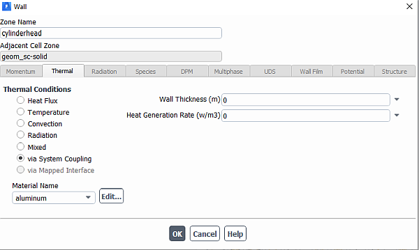
To couple the Fluent thermal analysis with Forte, the coupled boundaries cylinderhead and cylinderliner must be set as System Coupling boundaries, as shown in Figure 24.4: Enable System Coupling at the cylinderhead boundary condition in Fluent.
Normally, after the Fluent project is set up, you need to export the project
setting for System Coupling's use. To do this, navigate to File,
select Export → System Coupling → Write SCP File, and
save the project settings to an .scp file. In this tutorial, you do not
need this step, because the project settings have been saved to
fluent.scp and placed in the run directory. For more information about
how to prepare a Fluent project for System Coupling, refer to the Fluent User's Guide,
"Performing Command Line System
Coupling."
As mentioned, we have two participants for System Coupling, one is Forte with input variable Temperature and output variable Heat Rate, and the other is Fluent with input variable Heat Rate and output variable Temperature. The System Coupling setup is defined in the python script file named run.py. It invokes several functions, including loading the participants' project information, setting up the coupling interface, specifying both the control for coupled iterations and the options to promote convergence, and launching the simulation. The python script used in this tutorial is shown below as an example. You may use it as a template when setting up a new coupled simulation.
Example 24.1: run.py python script
import os

# Add Forte as coupling participant
forte = AddParticipant(InputFile = os.path.join('forte', 'Engine.ftsim'))

# Add Fluent as coupling participant
fluent = AddParticipant(InputFile = 'fluent.scp')


# Define coupling interfaces and data transfers
iName_1 = AddInterface(SideOneParticipant = fluent,
                       SideOneRegions = ['cylinderhead'],
                       SideTwoParticipant = forte,
                       SideTwoRegions = ['head'])

iheatrate_1 = AddDataTransfer(Interface = iName_1,
                              TargetSide = 'One',
                              SideOneVariable = 'heatflow',
                              SideTwoVariable = 'HEATR')

itemperature_1 = AddDataTransfer(Interface = iName_1,
                                 TargetSide = 'Two',
                                 SideOneVariable = 'temperature',
                                 SideTwoVariable = 'TEMP')

iName_2 = AddInterface(SideOneParticipant = fluent,
                       SideOneRegions = ['cylinderliner'],
                       SideTwoParticipant = forte,
                       SideTwoRegions = ['liner'])

iheatrate_2 = AddDataTransfer(Interface = iName_2,
                              TargetSide = 'One',
                              SideOneVariable = 'heatflow',
                              SideTwoVariable = 'HEATR')

itemperature_2 = AddDataTransfer(Interface = iName_2,
                                 TargetSide = 'Two',
                                 SideOneVariable = 'temperature',
                                 SideTwoVariable = 'TEMP')

dm = DatamodelRoot()
# Set maximum and minimum iterations and use ramping and relaxation to stablise convergence
dm.SolutionControl.MaximumIterations= 10
dm.SolutionControl.MinimumIterations= 1
dm.AnalysisControl.GlobalStabilization.Option='Quasi-Newton'
dm.AnalysisControl.GlobalStabilization.InitialRelaxationFactor=1
dm.CouplingInterface[iName_1].DataTransfer[iheatrate_1].Stabilization.Option = 'Quasi-Newton'
dm.CouplingInterface[iName_1].DataTransfer[iheatrate_1].Stabilization.InitialRelaxationFactor = 1
dm.CouplingInterface[iName_1].DataTransfer[iheatrate_1].ConvergenceTarget = 0.5

dm.CouplingInterface[iName_2].DataTransfer[iheatrate_2].Stabilization.Option = 'Quasi-Newton'
dm.CouplingInterface[iName_2].DataTransfer[iheatrate_2].Stabilization.InitialRelaxationFactor = 1
dm.CouplingInterface[iName_2].DataTransfer[iheatrate_2].ConvergenceTarget = 0.5

dm.ActivateHidden.BetaFeatures = True
dm.OutputControl.GenerateCSVChartOutput = True
dm.OutputControl.Option = 'EveryIteration'

# Launch the coupled simulation
Solve()
Here the first interface identifies the Fluent cylinderhead patch coupled with the Forte boundary condition head, while the second interface refers to Fluent patch cylinderliner coupled with the Forte boundary condition liner. We are transferring Forte's Heat Rate to Fluent's heatflow and Fluent's temperatures to Forte's boundary condition. Before starting the simulation is important to choose the appropriate coupling controls. In this tutorial the best practice makes use of the Quasi-Newton solution stabilization and acceleration method to transfer Heat Rate data from Forte to Fluent with an initial relaxation factor of 1 for both the interfaces with the intent to improve convergence (see "System Coupling Data Transfers" in the System Coupling User's Guide). The convergence targets for temperature data transfer are kept as the default, 0.01, while the ones for heat rate are loosened up to 0.5 for both coupled surfaces. A relaxation factor of 0.5 on temperature data transfer is set at the cylinder head interface to help with the stabilization. For post-processing purposes an Ansys EnSight output is generated by default at the end of the run, and the beta feature Generate CSV Chart Output has been activated.
To run System Coupling, you need to run the System Coupling python environment and pass the
run.py script.
On Windows, open a CMD prompt and type:
call "c:\Program Files\ANSYS Inc\v242\SystemCoupling\bin\systemcoupling" -t8 -R run.py
On Linux at the command prompt, type:
sh $home/ansys_inc/v242/SystemCoupling/bin/systemcoupling -t8 -R run.py
Note: If you changed the location of your Ansys install, change the path to v242 appropriately.
The System Coupling iterations will run until convergence is accomplished as defined in the python script. The coupled simulation converges in around 6 iterations under the current settings.
Once the coupled simulation has converged, you can examine the Forte and Fluent
simulation results in their directories. In the forte directory, you will
see a list of folders named as SCRun_<number>, where <number>
is the iteration number of the coupled simulation. Forte's simulation results in each
coupling step are stored in these folders.
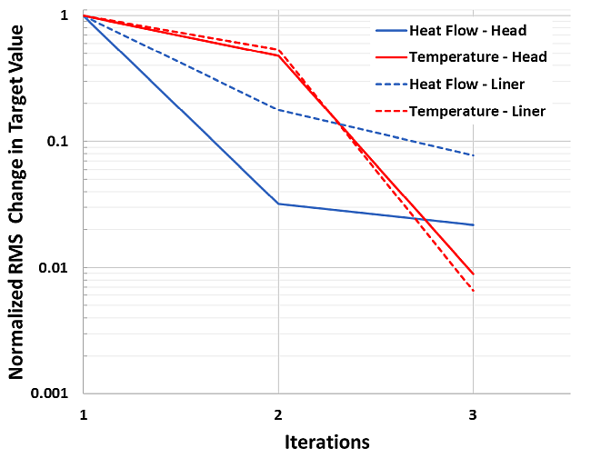
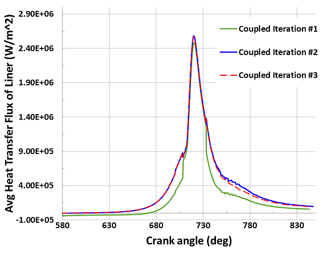
Figure 24.5: Averaged heat transfer flux on the engine cylinder liner as a function of crank angle in Forte shows, as an example, the spatially averaged wall heat transfer flux on the engine cylinder liner as a function of crank angle degree obtained from Forte at each iteration. As the coupled simulation proceeds, the heat transfer flux converges, due to a converging wall temperature boundary condition returned from System Coupling and applied on the cylinder liner.
Figure 24.5: Averaged heat transfer flux on the engine cylinder liner as a function of crank angle in Forte
To monitor and analyze the convergence status of the simulation, it is possible to activate in the run.py script the beta feature
DatamodelRoot().OutputControl.GenerateCSVChartOutput =
            True
and plot the normalized RMS change of data transferred at the coupling interface for both heat flow and temperature as in Figure 24.6: Forte's normalized RMS change in Target value: Heat flow and Temperature (further details about this beta feature can be found in the System Coupling Beta Features documentation). Note that the convergence target for heat flow data transfer for the cylinder head was set to 0.5 instead of the default value of 0.01, therefore the simulation can be considered converged.