The files for this tutorial are obtained by downloading the syc_fsi_oscillatingPlate.zip file here .

You have the opportunity to select the location for the files when you download and uncompress the sample files. Once downloaded and unpacked, they include:

This case uses 28 MPI processes and it typically completes (1 second of simulation time) in around 40 minutes on a dual Intel Xeon E5-2697v3 running at 2.59 GHz.

Before setting and launching the simulation, it is important to have the right folder structure in your own working directory. To accomplish this, follow these guidelines:

As mentioned, from the System Coupling viewpoint, there are two participants:

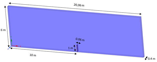
This tutorial simulates the oscillating plate within a fluid-filled cavity. Most of the project settings are similar to those of a stand-alone Forte simulation. The chemistry set used is the Air_NoReactions_2sp.cks, the turbulence model is the RNG k-ε model, and the mesh refinements follow the Forte Best Practices, available from the Forte page of the Ansys Help website.

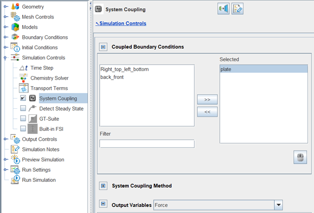
The global mesh size is set to 20 cm, and fixed refinements of 1/8^th of the global mesh size are applied to the plate. Gap refinements of the same fraction are applied to the front and back surfaces of the plate, to allow them to slide and block the flow passage with the front and back of the cavity. The cavity is fully filled by air at standard conditions, and it is closed so no inlet or outlet conditions need to be set. The plate position will be updated by Mechanical via System Coupling during the following iterations. To allow this and to send back updated force data to Mechanical, the System Coupling check box in the Simulation Control node must be activated as shown in Figure 22.3: Enable the System Coupling node, and the plate surfaces must be selected. Navigating through the System Coupling node, the Transient-Transient Coupling option is selected. Finally, the Force needs to be selected in the Output Variables panel.

Figure 22.3: Enable the System Coupling node

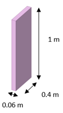
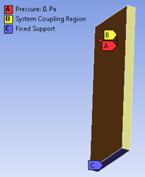
The transient structural analysis is performed in Mechanical. The geometry consists only of a vertical plate with a density of 2550 kg/m³, a Young's modulus of 2.5e6 Pa, and a Poisson's ratio of 0.3. When launching Ansys Workbench and unarchiving the Mech_OscPlate.wbpz project file, take a moment to explore the full setup (See Figure 22.4: Mechanical setup), and the mesh resolution. As you can see in the Model > Transient > Pressure node, there is an initial pressure of 100 Pa applied to the left surface of the plate for 0.5 seconds that will initiate the displacement of the plate. Verify that the plate sides and top surfaces are registered as System Coupling Region, and that the bottom of the plate is the Fixed Support of the plate.

Figure 22.4: Mechanical setup

If you happen to modify the Mechanical project, don't forget to write out the updated System Coupling settings file (*.scp) and the input file (*.dat).

To write the *.scp file, right-click to Transient and select Write System Coupling Files.

To write the *.dat file, click on Solution > Tools > Write Input File.

If you simply want to run the case as-is, the *.scp and *.dat files have already been generated and included in the downloaded files.

For more information about how to prepare a Mechanical project for System Coupling, refer to System Coupling in the Mechanical User's Guide.

The System Coupling setup is defined in the python script file named run.py. It invokes several functions, including loading the participants' project information, setting up the coupling interface, specifying both the control for coupled iterations and the options to promote convergence, and launching the simulation. The python script used in this tutorial is shown below as an example. You may use it as a template when setting up a new coupled simulation.

import os

# MAPDL is a Participant
mapdl = AddParticipant(InputFile = 'mapdl.scp')

# Forte is a Participant
forte = AddParticipant(InputFile = os.path.join('forte', 'Plate_SCFSI.ftsim'))

# Define coupling interface and data transfers
iName = AddInterface(SideOneParticipant = forte,
                     SideOneRegions = ['plate'],
                     SideTwoParticipant = mapdl,
                     SideTwoRegions = ['FSIN_1'])

iforce = AddDataTransfer(Interface = iName,
                TargetSide = 'Two',
                SideOneVariable = 'FORCE', 
                SideTwoVariable = 'FORC')

idisplacement = AddDataTransfer(Interface = iName,
                TargetSide = 'One',
                SideOneVariable = 'DISP', 
                SideTwoVariable = 'INCD')

# Set Time Steps
dm = DatamodelRoot()
dm.SolutionControl.EndTime =  '1 [s]'   
dm.SolutionControl.TimeStepSize = '0.1 [s]'  
# Set maximum and minimum iterations and use ramping to stablise convergence
dm.SolutionControl.MaximumIterations= 10  
dm.SolutionControl.MinimumIterations= 1
dm.AnalysisControl.GlobalStabilization.Option='Quasi-Newton'
dm.AnalysisControl.GlobalStabilization.InitialRelaxationFactor=1
dm.CouplingInterface[iName].DataTransfer[iforce].Stabilization.Option = 'Quasi-Newton'
dm.CouplingInterface[iName].DataTransfer[iforce].Stabilization.InitialRelaxationFactor = 1
dm.CouplingInterface[iName].DataTransfer[iforce].ConvergenceTarget = 0.05

dm.ActivateHidden.BetaFeatures = True
dm.OutputControl.GenerateCSVChartOutput = True
dm.OutputControl.Option = 'EveryStep'   

# Solve the coupled analysis
Solve()

The order in which the participants are started is given by the order in which they are listed in run.py, whereas the order of the interfaces is not important. The first interface identifies the Forte plate patch coupled with the Mechanical boundary FSIN_1 (note that these names are case sensitive). We are transferring Forte's Force (FORCE) to Mechanical's FORC and Mechanical's displacement (INCD) to Forte's boundary conditions (DISP). Before starting the simulation it is important to choose the appropriate coupling controls. In this tutorial the best practice sets to 10 the maximum iteration number per each time step to converge, and it makes use of the Quasi-Newton solution stabilization and acceleration method to transfer displacement data from Mechanical to Forte with no initial relaxation factor (see "System Coupling Data Transfers" in the System Coupling User's Guide). The convergence target for the displacement data transfer is kept as the default, 0.01, while it is set to 0.05 for the force. For post-processing purposes, an Ansys EnSight output is generated at each run (EveryStep), and the feature Generate CSV Chart Output has been activated. The simulation runs for 1 second with a 0.1 time step.