This tutorial describes a valved pulse-jet case using the Built-in Fluid Structure Interaction (FSI) in Ansys Forte CFD. This feature allows pressure loads from the fluid simulation to interact with boundaries causing them to translate or deform. Refer to the Forte User's Guide for a more detailed explanation of this feature.
This tutorial shows the application case of a pulsed jet with 8 reed valves, in which the flexing of the valves, modeled as cantilever beams, controls the flow passage between two communicating chambers.
The following sections describe:
This tutorial will cover all the set-up steps, but we recommend that you work through the Forte Quick Start Guide first and become familiar with the workflow of the Ansys Forte user interface.
The files for this tutorial are obtained by downloading the
fsi_pulse_jet.zip file
here
.
Note: The project file setup has been updated from previous releases. For release 2022 R1, get a release-specific download of the tutorial files from the Forte 2022 R1 page at the Ansys Help website.
Unzip the fsi_pulse_jet.zip to your
working folder.
Files provided in this tutorial include a Forte project file that has been fully configured as well as a set of facilitating input files that can be used to set up the Forte project starting from a blank project. Specifically, the files include:
valved_pulse_jet.ftsim: The fully configured Forte project file.
valved_pulse_jet.stl: The geometry file.
PulsedPressureProfile.csv: The inlet pulsed pressure profile.
Note: This tutorial is based on a fully configured sample project that contains the tutorial project settings. The description provided here covers the key points of the project set-up but is not intended to explain every parameter setting in the project. The project files have all custom and default parameters already configured; the text highlights only the significant points of the tutorial.
Forte may be launched in a command line mode to perform certain tasks such as preparing a run for execution, importing project settings from a text file, or various other tasks described in the Forte User's Guide. One of these tools allows exporting a textual representation of the project data to a text file.
Example
forte.sh CLI -project <project_name>.ftsim -export tutorial_settings.txt
Briefly, you can double-check project settings by saving your project and then running the command-line utility to export the settings in your tutorial project (<project_name>.ftsim), and then use the command a second time to export the settings in the provided final version of the tutorial. Compare them with your favorite diff tool, such as DIFFzilla. If all the parameters are in agreement, you have set up the project successfully. If there are differences, you can go back into the tutorial set-up, re-read the tutorial instructions, and change the setting of interest.
The working principle of a valved pulse jet consists of a sequence of pulse deflagrations in the main chamber that produces an increase of pressure and temperature and a consequent immediate gas expansion converted into thrust to propel a body. It is made of an intake section, the combustion chamber, and the exhaust pipe. Between the intake and the combustion chamber there is a thin sheet of metal to force the accelerated flow motion in a single direction. The thin sheet is generally cut into the shape of a stylized daisy with petals that widen towards their end. Each petal acts as a reed valve.
The valved pulse jet geometry used in this tutorial is illustrated in Figure 21.1: Valved pulse jet geometry. In order to focus on the Built-in Fluid Structure Interaction (FSI) feature, we decided not to model the exhaust pipe and to replace the sequence of pulse deflagrations with a pulsed pressure profile at the inlet. The profile is of a sinusoidal shape with a peak pressure of 6 bar. Looking at Figure 21.2: Exploded geometry, we see that the flow entering the diffuser is then split and accelerated by the conical cavity within the diffuser itself (in teal). It enters the connecting rings (in yellow) and hits the reed valves close to their tips. When the pressure from the diffuser is higher than the pressure in the main chamber the reed valves bend, and the flow enters the chamber. In contrast, when the flow from the diffuser has a lower pressure than the one in the chamber, the reed valves close to prevent back flow and force the flow toward the outlet. The flow is initialized everywhere with a pressure of 2 bar and a premixed composition. Specific dimensions and operating conditions are listed in Table 21.1: Dimensions and operating conditions.
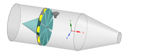
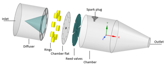
Table 21.1: Dimensions and operating conditions
| Item | Value | Units |
|---|---|---|
| Overall length | 35.2 | cm |
| Diffuser length | 9.76 | cm |
| Main chamber length | 24.7 | cm |
| Max diameter | 12 | cm |
| Number of reed valves | 8 | - |
| Premixed composition |
ch4 = 1 n2 = 7.52 o2 = 2 | Moles |
| Inlet pressure | pulsed profile | - |
| Outlet pressure | 2 | bar |
The project setup workflow follows the top-down order of the workflow tree in the Ansys Forte Simulate interface. The components irrelevant to the present project will not be mentioned in this document, and you can simply skip them and use the default model options.
Note: Changed values on any Editor panel do not take effect until you press the Apply button. Always press the Apply button after modifying a value, before moving to a new panel or the Workflow tree.
In this tutorial, we will import an existing geometry into Ansys Forte and set up the
automatic mesh generation using a global mesh size and adapting the mesh where extra
resolution is needed. To import the geometry, go to the Workflow tree and click
Geometry. This opens the Geometry icon bar.
Click the Import Geometry
 icon. In the resulting dialog, pull down and select Surfaces from one or more STL files, then select the provided STL
file, valved_pulse_jet.stl. In the dialog that opens with STL file
import options, accept the defaults. The mesh will be automatically generated during the
simulation. Note that once you have imported the geometry, there are a number of actions
that you can perform to modify the provided project on the items in the Geometry node, such
as scale, rename, transform, invert normals, or delete geometry elements. Use the
icon. In the resulting dialog, pull down and select Surfaces from one or more STL files, then select the provided STL
file, valved_pulse_jet.stl. In the dialog that opens with STL file
import options, accept the defaults. The mesh will be automatically generated during the
simulation. Note that once you have imported the geometry, there are a number of actions
that you can perform to modify the provided project on the items in the Geometry node, such
as scale, rename, transform, invert normals, or delete geometry elements. Use the ![]() button to fit the entire geometry in the graphic window.
button to fit the entire geometry in the graphic window.
To later allow easy identification of the bending direction of the reed, let us create one local reference frame for each valve. From the Geometry node, select Reference Frames and create the new reference frames. Their origins are indicated in Table 21.2: New reference frame origins in global coordinates.
Table 21.2: New reference frame origins in global coordinates
| Reference Frame (RF) | x | y | z | rotation about X-axis |
| Reed 1 | -8.36 cm | 0.205 cm | 0.414 cm | 334.09 deg |
| Reed 2 | -8.36 cm | -0.147 cm | 0.438 cm | 379.09 deg |
| Reed 3 | -8.36 cm | -0.414 cm | 0.205 cm | 424.09 deg |
| Reed 4 | -8.36 cm | -0.438 cm | -0.147 cm | 469.09 deg |
| Reed 5 | -8.36 cm | -0.205 cm | -0.414 cm | 514.09 deg |
| Reed 6 | -8.36 cm | 0.147 cm | -0.438 cm | 559.09 deg |
| Reed 7 | -8.36 cm | 0.414 cm | -0.205 cm | 604.09 deg |
| Reed 8 | -8.36 cm | 0.438 cm | 0.147 cm | 649.09 deg |
In the configured project that you previously downloaded, you can also see that a clip plane is created to allow a better view of the various components and reference frames, and a Sub-Volume region named Chamber.
The mesh creation occurs on-the-fly during the simulation, however, there are a few parameters that need to be set in the Mesh Controls node:
Material Point: This is needed to identify the simulation domain where the mesh will be generated. It should be located at least one unit cell length away from any boundaries and must be inside of the domain throughout the entire simulation. Set it at the Global Origin.
Global Mesh Size: Set the Global Mesh Size to 4 mm.
Refinements: These are needed to refine the mesh around key geometry features. They are of different types, those used in this tutorial are: Surface Refinement Depth, SAM (Solution Adaptive Mesh) , and Gap Feature Control. The Gap Feature Control automatically detects small gaps between the specified surface pair based on the user-specified Surface Proximity criterion and applies refinement in the detected gap region based on the user-specified refinement level. When Gap Feature Control is used, the spatially resolved solution will contain a variable called GapCellFlag, which uses non-zero integer values to mark the zones identified as gap zones. Detailed mesh control parameters are listed in Table 21.3: Settings for Mesh Control refinements.
Table 21.3: Settings for Mesh Control refinements
| Item | Refinement type | Refinement location | Refinement level | Refinement layers |
|---|---|---|---|---|
| Walls | Surface |
chamber, diffuser | 1/4 | 1 |
| Reeds | Surface |
chamber_flat, reed1_bottom, reed2_bottom, reed3_bottom, reed4_bottom, reed5_bottom, reed6_bottom, reed7_bottom, reed8_bottom | 1/4 | 4 |
| OpenBoundaries | Surface |
inlet, outlet | 1/4 | 1 |
| Rings_and_spark | Surface |
rings, spark_plug | 1/4 | 1 |
| SAMgradVel |
SAM Quantity Type = Gradient of Solution Field Solution Variables = VelocityMagnitude Bounds = Statistical Sigma Threshold = 0.1 | Sub-Volume: Chamber | 1/4 | - |
| SAMgradT |
SAM Quantity Type = Gradient of Solution Field Solution Varaibles = Temperature Bounds = Statistical Sigma Threshold = 0.1 | Sub-Volume: Chamber | 1/4 | - |
| Gapdepth X |
Gap Feature Surface Proximity = 0.05 cm Enable Gap Model = ON Gap Size Scale Factor = 1 |
chamber_flat, reedX_bottom | 1/16 | - |
Note: Although only 1 Gapdepth refinement is listed (for brevity), the Forte project file contains 8 of them. If your project is being set up starting from a blank project, do not forget to add the other 7, replacing X with the proper reed valve number ID.
All the settings in this node can be kept as the default, but don’t forget to import the provided chemistry set. Specifically:
Chemistry set: The chemistry input file used in this
tutorial is the default NaturalGas_1comp_29sp.cks and it can be found
in your Forte installation path inside the subfolder,
Program Files\ANSYS Inc\V242\reaction\forte.win64\data\. To use it, navigate to
the Chemistry module, click the ![]() icon and select the chemistry set,
NaturalGas_1comp_29sp.cks.
icon and select the chemistry set,
NaturalGas_1comp_29sp.cks.
Boundary conditions must be specified for each of the geometry elements. To match the provided project, follow these instructions for each boundary condition:
Inlet: Defined as an inlet boundary ![]() . Set the Mole Fraction Composition to be
1 ch4, 7.52
n2, and, 2 o2
and the location is inlet. Then select
Total Pressure, Time Varying, set Time as a
Time Option. Next to Pressure Profile select
Create new... and then click the button
. Set the Mole Fraction Composition to be
1 ch4, 7.52
n2, and, 2 o2
and the location is inlet. Then select
Total Pressure, Time Varying, set Time as a
Time Option. Next to Pressure Profile select
Create new... and then click the button ![]() . Once the Editor panel opens, click Load CSV to
upload the provided pressure profile (PulsedPressureProfile.csv). The
Total Temperature is 600 K and the Turbulence
parameters are kept at the default values.
. Once the Editor panel opens, click Load CSV to
upload the provided pressure profile (PulsedPressureProfile.csv). The
Total Temperature is 600 K and the Turbulence
parameters are kept at the default values.
Outlet: Defined as an inlet boundary ![]() , to force the reverse flow condition to be explicitly defined. Set the
Mass Fraction Composition as air, 0.24
o2 and 0.76
n2, and the location to be outlet.
The Total Pressure is set to 2 bar and the
Total Temperature to 350 K. Turbulence parameters
are kept at the default values.
, to force the reverse flow condition to be explicitly defined. Set the
Mass Fraction Composition as air, 0.24
o2 and 0.76
n2, and the location to be outlet.
The Total Pressure is set to 2 bar and the
Total Temperature to 350 K. Turbulence parameters
are kept at the default values.
Chamber: Defined as a wall boundary ![]() . The location selection lists center_ring,
chamber, chamber_flat. The Heat Transfer check
box is selected, the Wall Temperature is constant at
350 K, and the Heat Transfer Model in
use is the Han-Reitz Model.
. The location selection lists center_ring,
chamber, chamber_flat. The Heat Transfer check
box is selected, the Wall Temperature is constant at
350 K, and the Heat Transfer Model in
use is the Han-Reitz Model.
Diffuser: Defined as a wall boundary ![]() . The location selection lists the diffuser and the
rings. The Heat Transfer check box is selected,
and the Wall Temperature is constant at 600 K, and
the Heat Transfer Model in use is the Han-Reitz
Model.
. The location selection lists the diffuser and the
rings. The Heat Transfer check box is selected,
and the Wall Temperature is constant at 600 K, and
the Heat Transfer Model in use is the Han-Reitz
Model.
Spark: Defined as a wall boundary ![]() . The location selection lists only the spark_plug.
The Heat Transfer check box is selected, and the Wall
Temperature is constant at 450 K, and the Heat
Transfer Model in use is the Han-Reitz Model.
. The location selection lists only the spark_plug.
The Heat Transfer check box is selected, and the Wall
Temperature is constant at 450 K, and the Heat
Transfer Model in use is the Han-Reitz Model.
Then add the following boundary condition to each reed valve, replacing X with the number of each valve.
Reed X: Defined as a wall boundary ![]() . The location selections are reedX and
reedX_bottom. The Heat Transfer check box is NOT
selected.
. The location selections are reedX and
reedX_bottom. The Heat Transfer check box is NOT
selected.
The entire domain is initialized with the premixed composition listed in Table 21.1: Dimensions and operating conditions, and a constant Temperature and Pressure of 350 K and 2 bar, respectively.
The first setting in the Simulation Controls node is Time Based as the simulation option. Then set the Max. Simulation Time to be 2 ms.
Time Step: Only two parameters differ from the defaults to accommodate a larger time step without affecting much the accuracy and the stability of the solution. These are the Fluid Acceleration Factor, set to 2 and the Rate of Strain Factor, set to 2.4.
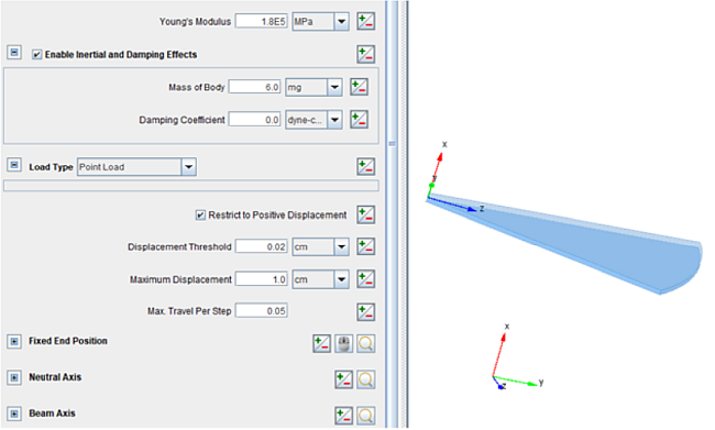
Built-in FSI : Activate the Built-in FSI
feature by checking the box, click the ![]() icon to create a new "Bending Beam" and name it Reed
1. Now, select the Reed 1 in the location list and choose
Point Load in the Load Type option. Assuming that
the reed valves are made of steel, set the Young's Modulus to
1.8e5 MPa. Select the Enable Inertial and Damping
Effects check box, and set the Mass of Body to be
6 mg. Then set the other parameters as shown in
Figure 21.3: Built-in FSI Bending Beam panel. The figure also shows the Reed 1
reference frame previously specified in Table 21.2: New reference frame origins in global coordinates; use it in the Fixed End
Position, the Neutral and Beam Axis
panels. The Fixed End Position specifies the origin of the beam and it corresponds to the
origin of the Reed 1 reference frame, so all the coordinates are set to 0
cm. Then the Neutral Axis is the direction along the main dimension of the beam,
set it to Z = 1 cm. Finally the Beam Axis is the
axis by which the beam will rotate, with positive deflection given by the right-hand rule,
set it to Y = 1 cm. Now repeat the above steps to
model for all the other valves as bending beams, making sure to replace each time their
selected location and the reference frames for the Fixed End Position, the Neutral and the
Beam Axes. In all the Bending Beams the Restrict to Positive
Displacement box is checked to constrain the valve motion. The Max.
Travel Per Step is set to 0.05. This represents the maximum
deflection of the beam as a fraction (5%) of the maximum displacement (1 cm) between mesh
updates.
icon to create a new "Bending Beam" and name it Reed
1. Now, select the Reed 1 in the location list and choose
Point Load in the Load Type option. Assuming that
the reed valves are made of steel, set the Young's Modulus to
1.8e5 MPa. Select the Enable Inertial and Damping
Effects check box, and set the Mass of Body to be
6 mg. Then set the other parameters as shown in
Figure 21.3: Built-in FSI Bending Beam panel. The figure also shows the Reed 1
reference frame previously specified in Table 21.2: New reference frame origins in global coordinates; use it in the Fixed End
Position, the Neutral and Beam Axis
panels. The Fixed End Position specifies the origin of the beam and it corresponds to the
origin of the Reed 1 reference frame, so all the coordinates are set to 0
cm. Then the Neutral Axis is the direction along the main dimension of the beam,
set it to Z = 1 cm. Finally the Beam Axis is the
axis by which the beam will rotate, with positive deflection given by the right-hand rule,
set it to Y = 1 cm. Now repeat the above steps to
model for all the other valves as bending beams, making sure to replace each time their
selected location and the reference frames for the Fixed End Position, the Neutral and the
Beam Axes. In all the Bending Beams the Restrict to Positive
Displacement box is checked to constrain the valve motion. The Max.
Travel Per Step is set to 0.05. This represents the maximum
deflection of the beam as a fraction (5%) of the maximum displacement (1 cm) between mesh
updates.
Note: During the simulation, each Bending Beam will generate two files with the extension
*_fsi.csv and *_displacements.csv. The first tracks the
Tip Deflection, the Load, the Pressure Force and the Torque applied to the valve versus time; while the other shows
the instantaneous deflection of the valve versus its neutral axis. Use Ansys Forte MONITOR to
see their evolution.
Output controls determine what data are stored for viewing during the simulation and for creating plots, graphs and animations in Ansys EnSight.
Spatially Resolved: Allows you to control when spatially resolved data such as velocity, temperature, pressure, etc., will be output. In the Spatially Resolved panel, set the Time Output Control to report every 0.1 ms. You can optionally increase the frequency of output to create smoother animations. Select then the Solution Count in the File Size Control and set the Solutions per Results File to 1 to have a single *.ftres per each output Time. Amongst the Spatially Resolved Species and Solution Variables, select variables of your interest like Pressure, Temperature, VelocityX, VelocityY, VelocityZ and Velocity Magnitude.
Spatially Averaged and Spray: Opt for Time and set the interval to 10 µs, then choose the species of interest if any.
Restart Data: This option allows a restart file to be saved at the end of the current simulation if the Write Restart File at Last Simulation Step option is checked. Such a restart file is useful if you decide to extend the simulation duration to do parameter studies because it provides a much better guess for initial condition than a uniform one.
Monitor Probes: Choose an Inquiry Frequency of 1 µs then create two monitor probes of type Geometric and shape Spherical with a 7 mm radius. Place them at 8 mm and -9 mm in the x-direction and 4.4 cm in the z-direction with respect to the Reed 3 reference frame and name them Chamber_sphere_reed3, and Diffuser_sphere_reed3, respectively. Let the probe output Pressure and Temperature.
To detect potential problems due to surface intersection and/or mesh generation before the
simulation is started, navigate to the Preview Simulation
node. On the Mesh Generation panel set the Time
Option to Time for investigating a specific Time
or to Time Range for a more extensive investigation, then
select Check for Surface Intersections and/or Include Volume Mesh depending on what you are interested in, and
finally launch the preview by clicking the
![]() icon. Due to the nature of this tutorial valves motion cannot be detected
with this preview since their motion is unknown ahead but depends on the flow simulation.
Nevertheless, the feature can be used to make sure all the other parts are behave as expected
and the volume mesh generation is appropriate.
icon. Due to the nature of this tutorial valves motion cannot be detected
with this preview since their motion is unknown ahead but depends on the flow simulation.
Nevertheless, the feature can be used to make sure all the other parts are behave as expected
and the volume mesh generation is appropriate.
The run settings depend on the system and environment for your simulations. Change the number of cores to use for this simulation according to the resources available to you by navigating to Run Settings > Run Options, and under Job Script Options, setting the number of cores for Default MPI Arguments. No other changes are needed, and you can proceed launching the simulation.
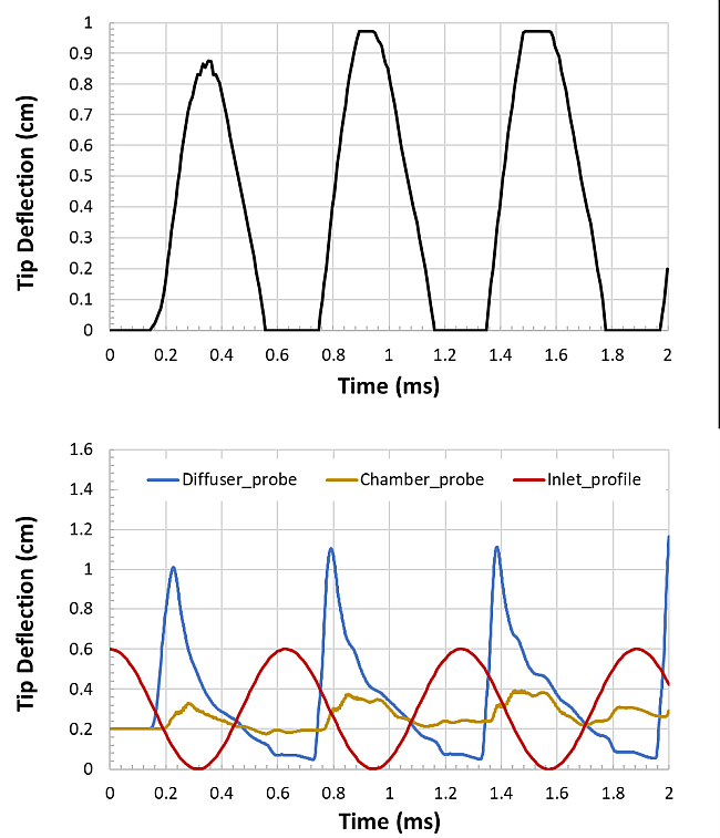
During the 2 ms simulation time the reed valves open synchronously 3 times. Figure 21.4: Tip deflection of Reed 3 at the top, spatially averaged chamber, diffuser probe pressure and pressure force felt by the reed at the bottom is an example of the tip deflection of the reed valve number 3 versus time. When the simulation starts, the pressure is 0.2 MPa everywhere, therefore a null pressure is applied to the valve and the valve remains in its closed position.
The pulsed pressure profile applied at the inlet (red line) determines the opening and closing of the daisy petal valves.
When the higher pressure reaches the proximity of the valve, the diffuser probe pressure rises (blue line) and becomes higher than the chamber's pressure (yellow line). Consequently, the pressure force applied to the reed increases and, at approximately 0.2 ms, causes the reed valve endpoints (black line) to bend toward the main chamber and open, allowing the flow to pass through. In contrast, at around 0.4 ms, the diffuser pressure becomes lower than the chamber pressure and forces the tip deflection of the valves to decrease and return to the initial closed position. The opening and closing cycle of the valves repeats until the end of the simulation, with maximum tip deflections slightly below 1 cm.
Figure 21.4: Tip deflection of Reed 3 at the top, spatially averaged chamber, diffuser probe pressure and pressure force felt by the reed at the bottom
In the Forte project file, we activated the gap resistance model within the Mesh Controls node as an option to the gap refinement control. We set it up to handle the evolving small gaps in-between the bottom of each valve and their seating surface, named chamber_flat. When the Gap Feature Control is used, the spatially resolved solution will contain a variable called GapCellFlag, which uses non-zero integer values to mark the zones identified as gap zones. In Figure 21.5: Evolution of the GapCellFlag on the valves' seating surfaces, and reed valves' deflection we can see their growth and shrinking reflected on the chamber_flat surface when the valves' deflection, and therefore the gap, change in time. To reproduce the dynamic plotting of the Deflection vs. Time on the top right, copy the first two columns of the Reed 3_fsi.csv file output from Forte without the column headers, and paste them into a new text file with the .exy format. Add 6 more rows as headers and fill them as follows:
1
Deflection vs. Time
Time
Deflection
1
Now in EnSight, click Create new Plot/Query. Select the option Read from an external file, and then select the file just created.
Figure 21.5: Evolution of the GapCellFlag on the valves' seating surfaces, and reed valves' deflection
Figure 21.6: Instantaneous pressure on reed valves during an opening/closing cycle reports the pressure change on the reed valves during their opening/closing cycle. At 0.8 ms the higher pressure in the diffuser starts hitting the valve tips, where red circles appear. The pressure difference between the diffuser and the main chamber keeps increasing and the flow exiting the connecting rings pushes the valves to full opening. As soon as that pressure difference decreases, and the diffuser pressure drops below the chamber pressure, at around 1.2 ms, the valves start closing and fully block the flow at 1.3 ms. The next opening cycle starts around 1.4 ms.
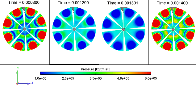
Figure 21.7: Contours evolution at a z-cut plane of pressure at top left, velocity magnitude with streamlines at bottom left, tip displacement at top right, and temperature at bottom right shows the pressure, velocity, and temperature distribution on a cut plane in the middle of the geometry. The animations reproduce the 3 full opening/closing cycle, in which the reed valves reach their maximum deflection and go back to their closed position. When valves are open, the hot flow is passing from the diffuser to the chamber. The back flow is then blocked as soon as the valves close. Note how the presence of the spark plug affects the flow and creates a stronger recirculation zone in the upper part of the domain. Similarly to Figure 21.5: Evolution of the GapCellFlag on the valves' seating surfaces, and reed valves' deflection, the deflection and time are in centimeters and seconds, respectively.
Figure 21.7: Contours evolution at a z-cut plane of pressure at top left, velocity magnitude with streamlines at bottom left, tip displacement at top right, and temperature at bottom right