This tutorial shows the simulation of a generic vane pump using Ansys Forte CFD. The vane pump belongs to the positive displacement pumps and allows the transfer of pressurized fluid. It consists of a rotor framed within a case, the working fluid is brought in through the suction port at low pressure, then while the rotor is turning, the vanes mounted on it slide in and out of their slots and form pockets of fluid delivered at higher pressure to the discharge port at a constant flow rate.
The following sections describe the provided files, time required, prerequisites, and a utility for comparing your generated project file (.ftsim) with the one provided in the tutorial download.
This tutorial will cover all the set-up steps, but we recommend that you work through the Forte Quick Start Guide first and become familiar with the workflow of the Ansys Forte user interface.
The files for this tutorial are obtained by downloading the
vane_pump_tutorial.zip file
here .
Unzip vane_pump_tutorial.zip to your working folder.
Files provided in this tutorial include a Forte project file that has been fully configured as well as a set of facilitating input files that can be used to set up the Forte project from scratch. Specifically, the files include:
Vane_Pump_Tutorial.ftsim: The fully configured Forte project file.
Vane_Pump_Surface_Geometry.stl: The surface geometry input file.
case_profile.csv: A list of points in cylindrical coordinates identifying the geometric profile of the case.
vane_pump_script.py: A python script to be run in Ansys Discovery script editor to extract the case_profile.csv if the geometry is modified.
All the files related to the UDF are collected inside a UDF_files subfolder:
fsi_user_defined_functions.cpp: The C++ coded UDF.
libForteUDF_fsi.dll: The already compiled, ready-to-use UDF for Windows systems.
libForteUDF_fsi.so: The already compiled, ready to use UDF for Linux systems.
ProjectData.hpp, fsi_user_defined_functions.hpp and LookupTable.h: Supporting UDF files.
HowToCompileTutorial_vanePump_UDF.txt: The text file containing instructions to recompile or modify the provided UDF.
The tutorial sample file is provided as a download. You have the opportunity to select the location for the file when you download and uncompress the sample files.
Note: This tutorial is based on a fully configured sample project that contains the tutorial project settings. The description provided here covers the key points of the project set-up but is not intended to explain every parameter setting in the project. The .ftsim file has all custom and default parameters already configured; the text highlights only the significant points of the tutorial.
The installation includes the cgns_util export command, which you can use to compare the parameter settings in the project file generated at any point during your tutorial set-up against the provided .ftsim, which has the parameter settings for the final, completed tutorial. This command is described in the Forte User's Guide.
Briefly, you can double-check project settings by saving your project and then running the cgns_util to export your tutorial project, and then to export the provided final version of the tutorial. Save both versions and compare them with your favorite diff tool, such as DIFFzilla. If all the parameters are in agreement, you have set up the project successfully. If there are differences, you can go back into the tutorial set-up, re-read the tutorial instructions, and change the setting of interest.
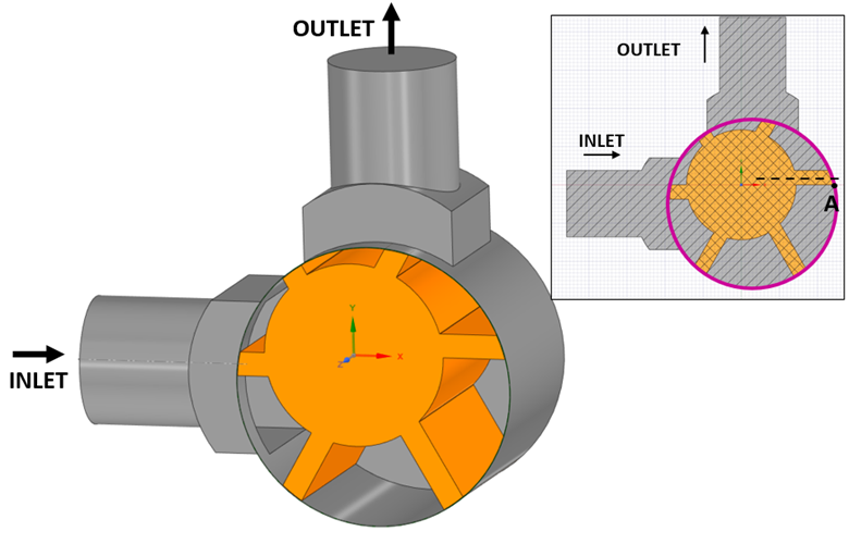
The generic vane pump described in this tutorial is shown in Figure 18.1: Vane pump geometry, 3D view and xy cut-plane, where the top part of the case embedding the rotor is made transparent to allow a better visualization of the inside. The working fluid is water, a pressure drop of 1.5 bar is applied between the inlet and outlet boundaries, with the inlet pressure set to 1 bar. The rotor has 6 vanes and rotates at 3000 RPM. As the rotor turns around the z-axis, the vanes go in and out of their slots. Generally, different mechanisms characterize the vanes in and out motion, in this tutorial the vanes simply slide in and out of the rotor with their tips following the profile of the side of the casing. The roto-translation of the vanes motion is controlled by the UDF. Please see UDF Walkthrough for further details on how to use, modify and compile the provided UDF. The pockets of fluid constrained by the vanes are transported toward the discharge port resulting in a smooth pumping action.
The project setup workflow follows the top-down order of the workflow tree in the Ansys Forte Simulate interface. The components irrelevant to the present project will not be mentioned in this document, and you can simply skip them and use the default model options.
One of the main advantages of using Forte in your simulation is that you don’t
need to create the volume mesh beforehand, since it will be automatically generated
on-the-fly. Instead, you only need to create a surface mesh and import it in
Forte. For this tutorial we provide the surface mesh in the
.stl format exported from the CAD geometry in Ansys Discovery, that
you need to import in the Forte UI. Go to the Geometry node
and click on Import Geometry ![]() , select the Surface from one or more STL
files option, pick your file or the
Vane_Pump_Surface_Geometry.stl and choose
cm as units. Note that once you have imported the geometry,
there are a number of actions that you can perform to modify the geometry elements,
such as scale, rename, transform, invert normals, or delete.
, select the Surface from one or more STL
files option, pick your file or the
Vane_Pump_Surface_Geometry.stl and choose
cm as units. Note that once you have imported the geometry,
there are a number of actions that you can perform to modify the geometry elements,
such as scale, rename, transform, invert normals, or delete.
Note: If you want to create the surface mesh yourself, we recommend using Fine and 4° for the Facet and Angle Resolution options, respectively, when exporting the .tgf file from Ansys Discovery. The reason being that the gear and casing geometries have curved surfaces in 3-D with tiny gaps in between, therefore the curved surfaces are required to be sufficiently smooth to avoid unwanted surface intersections during their motion. Another important check to perform when importing the surface mesh in Forte is to verify if the normal vectors of the triangulated surface mesh are pointing outward of the fluid domain. Generally, this is the case unless, as in this tutorial, you have nested volumes (the gears encapsulated inside the external case). So if you have created and imported your own geometry in Forte, select the rotor surfaces from the Geometry node, right-click and select Normals. This will turn on the normals to help you visualize if they are pointing inside the fluid domain. If that is the case, reselect those surfaces, right-click and choose Invert Normals
Note: For this tutorial we provide the geometry, but if you want to re-create or modify it with minimum changes to the UDF files, follow these rules:
Center the rotor at the Global Origin.
Let the z-axis be the rotation axis.
Draft all the vanes in their most retracted position.
Align the maximum radius of one of the vane tips with the x-axis (see point A in in Figure 18.1: Vane pump geometry, 3D view and xy cut-plane).
Allow that vane axis to be parallel to the x-axis (see dashed line in Figure 18.1: Vane pump geometry, 3D view and xy cut-plane).
Create a closed curve to identify the casing side (see the fuchsia pink circle in Figure 18.1: Vane pump geometry, 3D view and xy cut-plane). This is needed for the UDF to delimit the vanes extension. Further details can be found in UDF Walkthrough
Extract on a *.csv file the coordinates of the points of the closed curve just created. Keeping in mind that:
The points must be in cylindrical coordinates (theta, radius).
The first column must be the angle with respect to the x-axis (theta) and must be expressed in radians.
Theta should monotonically cover the entire period [0, 2pi] inclusively.
The second column must be the radius and must be expressed in centimeters.
OPTIONAL: you can use the provided vane_pump_script.py to extract the closed profile:
Open your geometry in Ansys Discovery.
Select Script Editor from the 3 lines menu at the very top left of the upper ribbon.
Load the vane_pump_script.py.
Modify the <MyPath> where you want your file to be saved.
Run it by clicking on the green arrow at the top right of the script window.
Your case_profile.csv file has been created.
To allow the mesh generation on-the-fly, you are required to setup the material point inside the fluid domain. For geometries with moving boundaries, like the one in this tutorial, you also want to make sure the material point will remain within the domain throughout the simulation. For this reason, we placed the material point next to the inlet boundary and away from any moving surfaces.
The coordinates of the Material Point are: x = -3 cm, y = -0.24 cm, z = -1.5 cm, and we chose a Global Mesh Size of 1 mm with static refinements applied as indicated in Table 18.1: Mesh refinements settings. The Active property is set to Always for all the mesh controls.
Among the Mesh controls there is an additional dynamic refinement type, the
Gap Feature Control ![]() , applied to the side of the casing and the each of the vanes.
In Table 18.1: Mesh refinements settings, see the specifics on the
refinement control marked as Vane X, where X stands for the vane number and goes
from 1 to 6. This type of refinement is of key importance when small gaps are
present. In its editor panel setting, you are asked to indicate a Surface
Proximity that will identify the gap between the pair of surfaces
selected in the Location box. For this tutorial we set the Surface
Proximity to be 0.2 mm for all the vanes and the
refinement level for those cells within the gap to ¼ of the
global mesh size.
, applied to the side of the casing and the each of the vanes.
In Table 18.1: Mesh refinements settings, see the specifics on the
refinement control marked as Vane X, where X stands for the vane number and goes
from 1 to 6. This type of refinement is of key importance when small gaps are
present. In its editor panel setting, you are asked to indicate a Surface
Proximity that will identify the gap between the pair of surfaces
selected in the Location box. For this tutorial we set the Surface
Proximity to be 0.2 mm for all the vanes and the
refinement level for those cells within the gap to ¼ of the
global mesh size.
Starting from 2024 R1, it is possible to modify the angular deviation between faces forming a gap. A value of zero indicates the faces bounding a gap must be parallel, a higher value is more permissive and will detect more gap cells. Due to the shape of the tips of the vanes, a Surface alignment threshold of 45 degrees is set to make sure the gap cells are correctly identified when the vanes move with the rotor.
In the same editor panel, check the Enable Gap Model box to compensate for the under-resolution in the gap zones. In other words, setting the refinement level to ¼ of the global mesh size, indicated that the fluid cells sizes within the gap are of 0.25 mm which means that some of the gaps only contain a fraction of a Cartesian cell cut by the physical boundary. Therefore, by enabling the Gap Model a momentum sink term is applied, which accounts for the underpredicted wall shear stress and over-predicted mass flow rate on the coarse grid. The Gap Model takes both the gap size and the local fluid cell size as inputs, and therefore the flow solution is not expected to be very sensitive to the gap refinement level.
The last parameter to set in the Gap Feature Control editor panel is the Gap Size Scale Factor. It can be used to enlarge or shrink the gap sizes measured on the geometry. The scaled gap size is then used as the input for the gap model in each local CFD cell in the gap zone. If the gap size in the geometry accurately reflects the size in the actual compressor, the best practice is to use the default value of 1.0. In this tutorial, we use the default value.
Table 18.1: Mesh refinements settings
| Refinement | Type | Location | Level | Layers |
|---|---|---|---|---|
| Casing | Surface |
bottom_case side_case top_case | 1/4 | 1 |
| OpenBoundaries | Surface |
inlet outlet | 1/2 | 2 |
| Vanes | Surface |
vane1 vane2 vane3 vane4 vane5 vane6 | 1/4 | 1 |
| Rotor | Surface |
bottom_rotor moving_tips_rotor side_rotor static_tips_rotor top_rotor | 1/4 | 1 |
| Ports | Surface |
discharge_port suction_port | 1/2 | 1 |
| Annulus | Annulusdepth |
Point 1: Ref. Frame: Global Origin X = 3.01, Y = -4.94, Z = 5 mm Point 2: Ref. Frame: Global Origin X = 3.01, Y = -4.94, Z = -35 mm Inner Radius 1 = 0.1 mm Outer Radius 1 = 23 mm Inner Radius 2 = 0.1 mm Outer Radius 2 = 23 mm | 1/2 | |
| Vane X | Gap Feature Surface Proximity = 0.2 mm Surface alignment threshold = 45 degrees Enable Gap Model = ON Gap Size Scale Factor = 1 |
side_case vaneX | 1/4 |
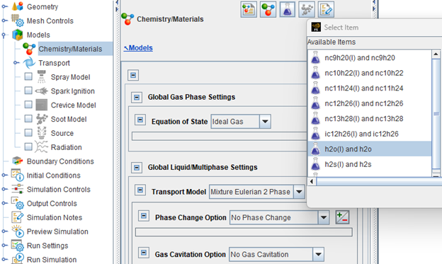
The working fluid in this vane pump tutorial is water, therefore it will be
sufficient to navigate to the Models >
Chemistry/Materials node, click on New Liquid and
Vapor Pair icon ![]() icon, and select h2o as shown in Figure 18.2: Liquid properties panel while keeping the default options. Once
you have picked your working fluid, you can use the Forte library liquid
properties. In this tutorial we have also added n2 and
o2 to the working fluid as shown in Figure 18.3: Inlet flow composition.
icon, and select h2o as shown in Figure 18.2: Liquid properties panel while keeping the default options. Once
you have picked your working fluid, you can use the Forte library liquid
properties. In this tutorial we have also added n2 and
o2 to the working fluid as shown in Figure 18.3: Inlet flow composition.
This tutorial uses the RANS RNG k-epsilon turbulence model, which is the default turbulence model option. Other turbulence modeling options are available under Models > Transport > Turbulence.
Boundary conditions must be specified for each of the surfaces found in the Geometry node. To match the provided project, follow these instructions for each boundary condition:
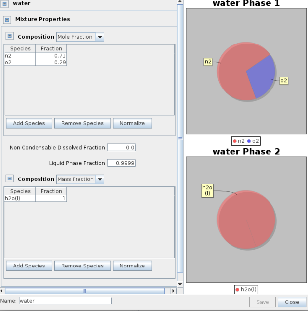
Inlet: Defined as an inlet boundary
 . To be able to consider liquids as part of the inlet
flow, Create a new multiphase mixture as shown in Figure 18.3: Inlet flow composition, and let the Liquid
Phase Fraction to be 0.9999, so that a small
amount of air can be present in the working fluid. Save the mixture. Then
pick the inlet surface as the selected
Location, set the Static Pressure
to 1 bar, leave the Turbulent Kinetic
Energy and Length Scale at their default
values, and finally set the Static Temperature to
300 K.
. To be able to consider liquids as part of the inlet
flow, Create a new multiphase mixture as shown in Figure 18.3: Inlet flow composition, and let the Liquid
Phase Fraction to be 0.9999, so that a small
amount of air can be present in the working fluid. Save the mixture. Then
pick the inlet surface as the selected
Location, set the Static Pressure
to 1 bar, leave the Turbulent Kinetic
Energy and Length Scale at their default
values, and finally set the Static Temperature to
300 K.Outlet: Defined as an inlet boundary
, to allow imposing the composition and temperature to
the reverse flow. Pick the outlet surface as
Location and use the same water
composition as the one at the inlet. Set the Static
Pressure to Time Varying, and let it ramp up
from 1 bar to 2.5 bar in
1.5 ms. This ramping profile helps reduce pressure
fluctuation at the beginning of the simulation. Then, leave the
Turbulent Kinetic Energy and Length
Scale at their default values, and finally set the
Static Temperature to 300
K.
In the Initial Conditions under Default Initialization use the same as the inlet oil composition in Figure 18.3: Inlet flow composition. Set the Temperature to 300 K, the Pressure to 1 bar, the Turbulent Kinetic Energy and Length Scale to their default values.
Let the simulation to be Time Based and enter the Max. Simulation Time of 20 msec (1 revolution). Leave everything else as default.
In the Time Step editor panel, set the Initial Simulation Time Step to be 5e-7 sec, and the Max. Simulation Time Step to be 5e-5 sec. Then, in the Advanced Time Step Control Options set the Fluid Acceleration Factor to be 1 and the Rate of Strain Factor to be 1.2.
In the Chemistry Solver editor panel, turn off chemistry by setting Activate Chemistry to Always Off.
For the Transport Terms controls we recommend using 1e-5 as the Pressure Iteration Tolerance as for all cases where liquids or 2-phase flows are involved in the simulation.
The motion of the sliding vanes is controlled by a UDF. To turn it on, enable
the Built-in FSI check box, and then click on the
New UDF icon ![]() and label it Vanes_UDF. In the
Editor Panel > UDF Library, browse to
the location where you previously stored the dynamically linked library
(*.dll for Windows OS and *.so for
Linux OS) provided with this tutorial. Select the boundary condition associated
with the Vanes, and make sure to have the Global
Origin set as the coordinate system used by the UDF. If you want to
recompile or modify the .cpp source file, follow the
instructions listed in the
HowToCompileTutorial_vanePump_UDF.txt file provided with
this tutorial.
and label it Vanes_UDF. In the
Editor Panel > UDF Library, browse to
the location where you previously stored the dynamically linked library
(*.dll for Windows OS and *.so for
Linux OS) provided with this tutorial. Select the boundary condition associated
with the Vanes, and make sure to have the Global
Origin set as the coordinate system used by the UDF. If you want to
recompile or modify the .cpp source file, follow the
instructions listed in the
HowToCompileTutorial_vanePump_UDF.txt file provided with
this tutorial.
It is recommended to store the provided dynamic library inside your C:\Program Files\ANSYS Inc\vXXX\reaction\forte.win64\user_defined_functions\bin folder.
It is recommended to perform a preview of the mesh from the node Preview Simulation > Mesh Generation to make sure there are no intersections when the rotor turns, and the vanes slides in and out.
The provided fsi_user_defined_functions.cpp includes multiple commented lines and helper functions that will aid understanding the written code while providing further examples of general useful operations to modify the UDF itself. Take the time to go through it, below we are focusing on the key sections of this UDF.
Before diving into the details of the UDF, make sure you have already created (or simply downloaded) the case_profile.csv file. When running the simulation, this file needs to be placed at the location indicated on line #415 for Windows runs and #417 for Linux ones in the fsi_user_defined_functions.cpp file. To use the UDF as is, place the case_profile.csv next to the Forte project *.ftsim file, the LookupTable.h will read it in and will use it as a constraint for the vanes extension motion.
In the same *.cpp file, have a look at the Forte_UDF_FSI_Initialize_Surface_Mesh method. Gathered here is information about the initial topology of the surface mesh; vertices and triangular facets associated with this UDF instance are identified. As mentioned earlier in Prepare and Import the Surface Geometry, the rotor is turning around the +z axis and it is counting 6 vanes (lines #424 and #425). The initial angle of the first vane with respect to the max radius point about the z-axis from the x-axis is 0° (line #430).
After that, the method Forte_UDF_FSI_Set_Load is called once per UDF update cycle. It provides fields values associated with the previously identified vertices. When running the simulation, a message will print out in the MONITOR file (line #526) the “Area integral of Pressure”.
The Forte_UDF_FSI_Get_Updated_Vertices is where the vertex locations are updated for the specified boundary once per UDF update cycle. It is important here too, to specify the hardcoded values of:
the axis of rotation (line #559),
the number of vanes (line #560),
the angle of the first vane's max radius location in the initial position of the rotor (line #564),
the angle the vane slides with respect to the radial direction (line #567),
the distance of the first vane's max radius in the initial position from the center of rotation (line #569),
the angular velocity of the rotor (line #571)
Once these values are set, the current rotation angle is retrieved, the offset table is interrogated, and the vanes are rotated and translated accordingly one at the time.
Output controls determine what data are stored for viewing during the simulation and for creating plots, graphs and animations in Ansys EnSight.
Spatially Averaged and Spray: Opt for Time in the Spatially Averaged Output Control and set the interval to 1e-6 sec, then choose the species of interest if any. In the editor panel, check the Enable Pocket Tracking box, leave the Minimum Pocket Volume Fraction at its default value, and adjust the Maximum Number of Tracked Pocket to 12. Forte will dynamically track contiguous pockets of fluid in the domain. The pockets are fluid volumes separated by gap cells. The pockets are marked using a variable called pocket_index in Spatially-Resolved solution. Spatially-Averaged pressure and total volume of each tracked pocket are reported in pocket_tracking.csv. For these types of pumps, it is handy to estimate time averaged outputs such as the mass flow rate at the outlet. Check the Enable Time Averaging Output box at the bottom of the editor panel and pick the Time Averaging Option of your choice. It is good practice to discard the first revolution and start averaging after that. In this tutorial we only simulate 1 revolution, so we keep the default option of Use All Time Points.
Restart Data: It is good practice to enable the restart data writing at the end of a simulation in case you want continue it later. You could also choose to have restart files written at a certain frequency or at specified times depending on your needs.
Additional Output: Starting with Ansys Forte 2022 R1, alongside the standard spatially resolved outputs (.ftres format), Forte offers the possibility to have an additional or an alternative set of output format, namely EnSight DVS (Dynamic Visualization Store). The DVS format helps reduce the loading time and the stepping through transient solution points in Ansys EnSight, thanks to the smaller size of the files generated. Better performance is also expected during the solution writing, especially when running a job on a cluster with many processors. To utilize the EnSight DVS format, start by clicking the EnSight icon on the Additional Output editor panel. Then check the Enabled box under EnSight DVS Settings. The output settings follow the same structure as Forte's native spatially resolved outputs. In other words, select your Interval Based Output Control frequency and pick your Solution Variables of interest. Only those in this list will be found in EnSight, so it is always suggested to have amongst this at least Pressure and Velocity Magnitude. If you scroll down in the same EnSight DVS editor panel you can also add the Spatially Averaged Datasets in the same additional output files set.
Note: If you fail to select the Enabled box, no EnSight DVS output will be generated, even if the rest of the panel is properly set. DVS output can be enabled independently from Forte's spatially resolved output. Therefore it often makes sense to disable Forte's spatially resolved output when using DVS.
The DVS results will be contained in a subfolder of the run directory, named according to the user-supplied name of the DVS output added to the Workflow tree. To load the results in EnSight, within an EnSight session, choose File > Open and select the .dvs file from this directory or use the EnSight launcher shortcut on Forte's Run panel, which will search for and provide a list of available .dvs files in the analysis directory that can be preselected and passed to the newly launched EnSight instance.
To detect potential problems due to surface intersection or mesh generation before the
simulation is started, navigate to the Preview Simulation node. On
the Mesh Generation panel, set the Time Option
to Time for investigating a specific Time or
to Time Range for a more extensive investigation, then select
Check for Surface Intersections and/or Include Volume
Mesh (highly recommended for a case with moving parts), and finally launch
the preview by clicking the Generate Mesh ![]() icon. Due to the nature of this tutorial, it is a good idea to
create a mesh preview with multiple steps spanning over an entire revolution to check
the mesh quality across the full rotation. In the Mesh Generation editor panel, you can
also select how many cores to use when performing this mesh check by changing the
MPI Arguments under the Run Options.
icon. Due to the nature of this tutorial, it is a good idea to
create a mesh preview with multiple steps spanning over an entire revolution to check
the mesh quality across the full rotation. In the Mesh Generation editor panel, you can
also select how many cores to use when performing this mesh check by changing the
MPI Arguments under the Run Options.
Note: For a quick check on the UDF motion, generate a mesh preview without enabling the Check for Surface Intersections and Include Volume Mesh options. This will provide a similar output to the one shown in Figure 18.4: Preview simulation output.
The run settings depend on the system and environment for your simulations. Change the number of cores to use for this simulation according to the resources available to you by navigating to Run Settings > Run Options, and under Job Script Options, setting the number of cores for Default MPI Arguments. No other changes are needed, and you can continue launching the simulation.
Note: This simulation runs in isothermal mode, therefore the environment variable FORTE_ISOTHERMAL=1 needs to be set under Windows Settings (or Linux Settings) > Environment Variable.
The final section of this tutorial is a collection of the results. In Figure 18.5: Pressure, velocity magnitude, volume mesh, and pocket ID evolution (time is in seconds), you can see on the left side of the view, the evolution of pressure and velocity along a cut plane in the middle of the z-direction. The ports are made transparent to allow a visualization of the inside and at the same time maintain the 3-dimensionality of the problem. In the animated GIF, notice how the mesh generated on-the-fly keeps changing to follow the motion of the rotor and its vanes at the top right view of the figure. At the bottom right of the GIF, the same clip plane is colored with the pocket index IDs. The ports volumes have ID #1 and #2; starting with ID #3 up to #10, iso-volumes of pocket Index are created to better show how each pocket is evolving.
Figure 18.5: Pressure, velocity magnitude, volume mesh, and pocket ID evolution (time is in seconds)
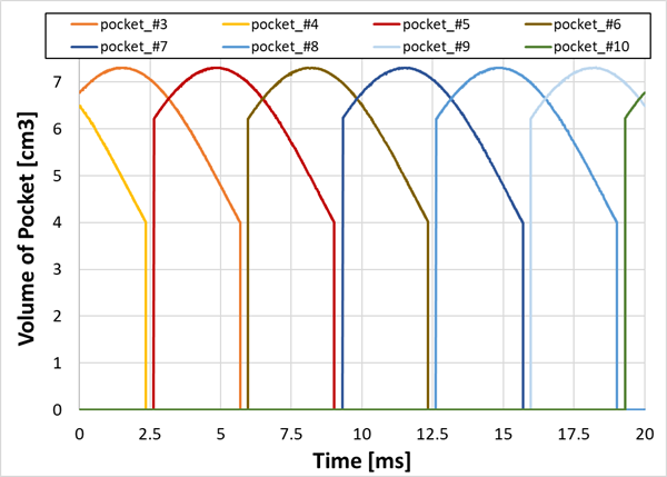
To look at the pockets all together, amongst the spatially averaged .csv output you may have noticed the presence of a file named pocket_tracking.csv. This output is generated only if the Pocket Tracking option is enabled under Spatially Averaged And Spray Output Controls as specified in Output Controls. If you open this file and plot the volume of each pocket, you will get a similar graph to the one reported in Figure 18.6: Volume of Pockets evolution. Amongst the 12 recorded pockets, there are also 2 OPEN pockets (#1 and #2 not reported in this graph), those represent the suction and discharge ports as previously mentioned. The other pockets of fluid are created and extinguished multiple times during the simulation. Pockets number #11 and #12 are also not shown since they are not yet formed at the end of the 1st revolution. It is worth noting that only 2 pockets coexist at the same time (excluding the OPEN pockets).
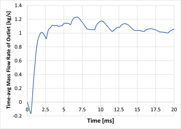
In the design phase of a vane pump, the mass flow rate of the outlet plays an important role, therefore we report its trend in time in Figure 18.7: Spatially and Time-averaged mass flow rate of outlet vs. time.