This tutorial shows the simulation of a generic gerotor pump using Ansys Forte CFD. The gerotor name is the shorter version of the generated rotor, and it belongs to the category of positive displacement pump family. It consists of a simple design with mainly two components: an inner driving gear, and an outer driven one, also called the idler. The idler is provided with an extra tooth with respect to the embedded inner rotor and has its center line positioned at a fixed eccentricity from the center line of the inner rotor and shaft. The gears can operate in either direction and allow the fluid entering from the suction port to be compressed and displaced smoothly toward the discharge port. The locked liquid pockets in between gears assure a good control over the volume of fluid travelling outside of the pump on each revolution.
The following sections describe the provided files, time required, prerequisites, and a utility for comparing your generated project file (.ftsim) with the one provided in the tutorial download.
This tutorial will cover all the set-up steps, but you should work through the Forte Quick Start Guide first and become familiar with the workflow of the Ansys Forte user interface.
The files for this tutorial are obtained by downloading the
generic_gerotor_tutorial.zip file
here
.
Unzip generic_gerotor_tutorial.zip to your working folder.
Note: For 2024 R1, the project file set-up has been updated from previous releases. The previous release, 2022 R1, requires a release-specific download of the tutorial files from the Forte 2022 R1 page at the Ansys Help website.
Files provided in this tutorial include a Forte project file that has been fully configured as well as a set of facilitating input files that can be used to set up the Forte project starting from a blank project. Specifically, the files include:
Generic_Gerotor_Tutorial.ftsim: The fully configured Forte project file.
Generic_Gerotor_Suface_Geometry.stl: The geometry file.
The tutorial sample compressed archive is provided as a download. You have the opportunity to select the location for the file when you download and uncompress the sample files.
Note: This tutorial is based on a fully configured sample project that contains the tutorial project settings. The description provided here covers the key points of the project set-up but is not intended to explain every parameter setting in the project. The project files have all custom and default parameters already configured; the text highlights only the significant points of the tutorial.
Forte may be launched in a command line mode to perform certain tasks such as preparing a run for execution, importing project settings from a text file, or various other tasks described in the Forte User's Guide. One of these tools allows exporting a textual representation of the project data to a text file.
Example
forte.sh CLI -project Generic_Gerotor_Tutorial.ftsim -export tutorial_settings.txt
Briefly, you can double-check project settings by saving your project and then running the command-line utility to export your tutorial project's settings, and then to export the provided final version of the tutorial's settings. Compare them with your favorite diff tool, such as DIFFzilla. If all the parameters are in agreement, you have set up the project successfully. If there are differences, you can go back into the tutorial set-up, re-read the tutorial instructions, and change the setting of interest.
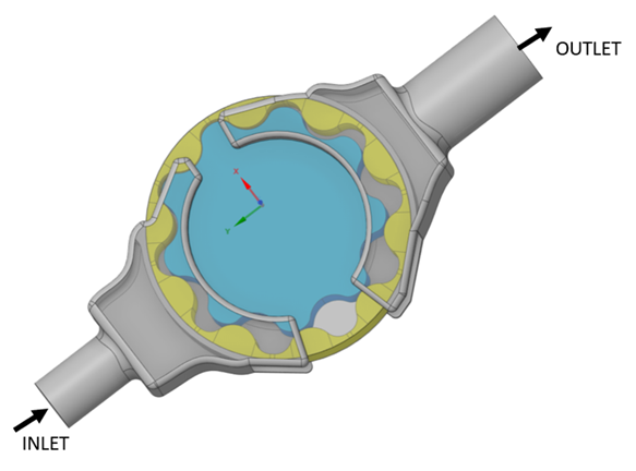
The generic gerotor described in this tutorial is shown in Figure 17.1: Generic gerotor geometry realized with Ansys SpaceClaim, where the case embedding the gears and the top of the ports are made transparent to allow a better visualization of the inside, and the working fluid is oil. A pressure drop of 4 atm is applied between the inlet and outlet boundaries, with the inlet pressure being equal to atmospheric. The light blue gear has 9 teeth and rotates at 2000 RPM while the yellow gear has 10 teeth and rotates at 1800 RPM. The inner RPM speed is generally part of the specifications of such pumps, while the speed of the external gear is calculated by dividing the number of teeth of the inner gear by those of the outer gear and then multiplying it by the RPM of the internal rotor. As the inner gear rotates, gaps between the rotors expand, trap fluid into them, and carry it toward the discharge port. The result is a smooth pumping action.
The project setup workflow follows the top-down order of the workflow tree in the Ansys Forte Simulate interface. The components irrelevant to the present project will not be mentioned in this document, and you can simply skip them and use the default model options.
Note: Changed values on any Editor panel do not take effect until you press the Apply button. Always press the Apply button after modifying a value, before moving to a new panel or the Workflow tree.
One of the main advantages of using Forte in your simulation is that you don't need
to create your volume mesh beforehand, since it will be automatically generated on-the-fly.
Instead, you only need to create a surface mesh and import it into Forte. For this
tutorial Ansys provides the surface mesh in the .stl format exported
from the CAD geometry in Ansys SpaceClaim, that you need to import in the Forte user
interface. Go to the Geometry node and click Import
Geometry![]() , select the option Surface from one or more STL
files, pick your file or the
Generic_Gerotor_Surface_Geometry.stl and choose cm
as the units. Note that once you have imported the geometry, there are a number of actions
that you can perform to modify the geometry elements, such as scale, rename, transform,
invert normals, or delete.
, select the option Surface from one or more STL
files, pick your file or the
Generic_Gerotor_Surface_Geometry.stl and choose cm
as the units. Note that once you have imported the geometry, there are a number of actions
that you can perform to modify the geometry elements, such as scale, rename, transform,
invert normals, or delete.
Before moving away from the geometry module, let us create a customized reference frame
to use in setting up the rotation axis of the outer gear. Under
Geometry > Reference Frames, click the
New Reference Frame icon ![]() and name it Center_OuterGear. Now, place its
origin at X = -3.266 mm, Y = -0.2965 mm,
Z = -41.7 mm, and accept the same orientation as the global origin.
and name it Center_OuterGear. Now, place its
origin at X = -3.266 mm, Y = -0.2965 mm,
Z = -41.7 mm, and accept the same orientation as the global origin.
Note: If you want to create the surface mesh yourself, Ansys recommends using the option
Fine and 4° for the
Facet and
AngleResolution, respectively, when exporting
the .tgf file from Ansys SpaceClaim. This is because the gears and
casing geometries have curved surfaces in 3-D, with tiny gaps in between, therefore the
curved surfaces must be sufficiently smooth to avoid unwanted surface intersections during
their motion. Another important check to perform when importing the surface mesh in
Forte is to verify if the normal vectors of the triangulated surface mesh are pointing
outward of the fluid domain. Generally this is the case, unless, as in this tutorial, you
have nested volumes (the gears encapsulated inside the external case). So if you have
created and imported into Forte your own geometry, select the
outer and innergears
surfaces from the Geometry node, right-click and select Normals. This
will turn on the Normals to help you visualize whether the normals are pointing to the
inside of the fluid domain. If that is the case, reselect those surfaces, right-click and
![]() .
.
To allow the mesh generation to proceed on-the-fly, you are required to set up the material point inside the fluid domain. For geometries with moving boundaries, like the one in this tutorial, you also must ensure that the material point will remain within the domain throughout the simulation. For this reason, we placed the material point next to the inlet boundary and away from any moving surfaces.
The coordinates of the Material Point are: X = -0.3 cm, Y = 8.5 cm, Z = -4.0 cm, with a Global Mesh Size of 2.5 mm with static refinements applied as indicated in Table 17.1: Mesh refinement settings. The Active property is set to Always for all the mesh controls.
Among the mesh controls there is an additional dynamic refinement named
Gears of the type Gap Feature Control ![]() , applied to the side of the gears facing each other:
inner_gear_side and outer_gear_inside. This type
of refinement is of key importance when small gaps are present. In its editor panel setting,
you are asked to indicate a Surface Proximity that will identify the
gap between the pair of surfaces selected in the Location box. For this
tutorial we set the Surface Proximity to be 0.7
mm. This value should be slightly bigger than the local cell size before the gap
refinement level of 1/8 is applied. So if the global mesh size is 2.5 mm and the local cell
size is 1/4 of that (0.625 mm) the value of 0.7 mm is a valid estimate.
, applied to the side of the gears facing each other:
inner_gear_side and outer_gear_inside. This type
of refinement is of key importance when small gaps are present. In its editor panel setting,
you are asked to indicate a Surface Proximity that will identify the
gap between the pair of surfaces selected in the Location box. For this
tutorial we set the Surface Proximity to be 0.7
mm. This value should be slightly bigger than the local cell size before the gap
refinement level of 1/8 is applied. So if the global mesh size is 2.5 mm and the local cell
size is 1/4 of that (0.625 mm) the value of 0.7 mm is a valid estimate.
In the same editor panel, check the Enable Gap Model box to compensate for the under-resolution in the gap zones. A momentum sink term will be applied to account for the underpredicted wall shear stress and overpredicted mass flow rate on the coarse grid. The Gap Model takes both the gap size and the local fluid cell size as inputs, and therefore the flow solution is not expected to be very sensitive to the gap refinement level.
The last parameter to set in the Gap Feature Control editor panel is the Gap Size Scale Factor. It can be used to enlarge or shrink the gap sizes measured on the geometry. The scaled gap size is then used as the input for the gap model in each local CFD cell in the gap zone. If the gap size in the geometry accurately reflects the size in the actual compressor, the best practice is to use the default value of 1.0. In this tutorial, we shrank the original inner gear CAD geometry to avoid potential surface intersection between the gears. Therefore, we set the Gears gap size scale factor to 0.3 and the *_bottomCase gap values to 0.5 to reduce flow leakage through those gaps in the simulation. When using simulation to guide gerotor design, this Gap Size Scale Factor also allows you to study the impact of gap size on simulation results without needing to modify the geometry itself.
See Table 17.1: Mesh refinement settings for a complete list of all the refinements.
Table 17.1: Mesh refinement settings
| Refinement | Type | Location | Level | Layers |
|---|---|---|---|---|
| OpenBoundaries | Surface |
inlet outlet | 1/2 | 2 |
| Ports | Surface |
exhaust intake | 1/2 | 1 |
| Walls | Surface |
bottom_case inner_gear_bottom inner_gear_side inner_gear_top outer_gear_bottom inner_gear_inside outer_gear_outside outer_gear_top side_case top_case | 1/4 | 1 |
| Case | Annulus |
Point 1: Ref. Frame: Center_OuterGear X = 0, Y = 0, Z = -1.5 cm Point 2: Ref. Frame: Center_OuterGear X = 0, Y = 0, Z =1.5 cm Inner Radius 1 = 2.0 cm Outer Radius 1 = 4.5 cm Inner Radius 2 = 2.0 cm Outer Radius 2 = 4.5 cm | 1/4 | _ |
| Gears |
Gap Surface Proximity = 0.7mm Gap Size Scale Factor = 0.3 | inner_gear_side outer_gear_inside |
1/8 | |
| innerGear_topCase |
Gap Surface Proximity = 0.7mm Gap Size Scale Factor = 1 |
inner_gear_top top_case | 1/4 | |
| outerGear_topCase |
Gap Surface Proximity = 0.7mm Gap Size Scale Factor = 1 |
outer_gear_top top_case | 1/4 | |
| innerGear_bottomCase |
Gap Surface Proximity = 0.7mm Gap Size Scale Factor = 0.5 |
bottom_case inner_gear_bottom
| 1/4 | |
| outerGear_bottomCase |
Gap Surface Proximity = 0.7mm Gap Size Scale Factor = 0.5 |
bottom_case outer_gear_bottom
| 1/4 |
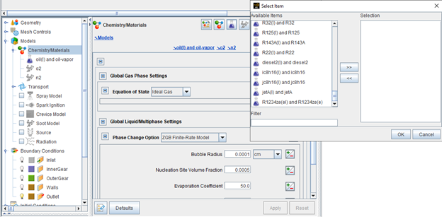
The working fluid in this generic gerotor is oil, therefore navigate to the
Models > Chemistry/Materials node, click the
New Liquid and Vapor Pair icon ![]() and add oil(l) and oil-vapor. Once you have
selected your working fluid, you can either use the Forte library liquid properties or
modify the database values. In this case, select User Defined Values
for Liquid Properties, then select Override the Database
Liquid Density, Viscosity, and Vapor Pressure with
Constant Values. We set the Density to 882
kg/m3, the Viscosity to 2.047e-3
kg/m-sec, and the Vapor Pressure to 400
Pa. To make the working fluid more realistic, we have also added a small amount
of air, therefore n2 and o2 are added as gaseous components.
and add oil(l) and oil-vapor. Once you have
selected your working fluid, you can either use the Forte library liquid properties or
modify the database values. In this case, select User Defined Values
for Liquid Properties, then select Override the Database
Liquid Density, Viscosity, and Vapor Pressure with
Constant Values. We set the Density to 882
kg/m3, the Viscosity to 2.047e-3
kg/m-sec, and the Vapor Pressure to 400
Pa. To make the working fluid more realistic, we have also added a small amount
of air, therefore n2 and o2 are added as gaseous components.
Now, as shown in Figure 17.2: Liquid Properties panel, keep the default Ideal Gas and select the ZGB Finite-Rate Model method to model the Phase Change.
This tutorial uses the RANS RNG k-epsilon turbulence model, which is the default turbulence model option. Other turbulence modeling options are available under Models > Transport > Turbulence.
Boundary conditions must be specified for each of the surfaces found in the Geometry node. To match the provided project, follow these instructions for each boundary condition:
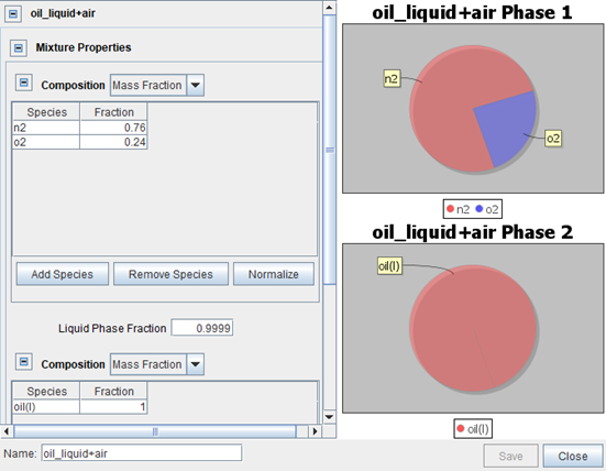
Inlet: Defined as an inlet boundary ![]() . To be able to consider liquids as part of the inlet flow,
Create a new multiphase mixture as shown in
Figure 17.3: Inlet flow composition, and allow the Liquid Phase
Fraction to be 0.9999. Save the mixture. Then pick the
inlet surface as the selected Location, set the
Static Pressure to 1 atm, leave the
Turbulent Kinetic Energy and Length Scale at their
default values, and finally set the Static Temperature to 300
K.
. To be able to consider liquids as part of the inlet flow,
Create a new multiphase mixture as shown in
Figure 17.3: Inlet flow composition, and allow the Liquid Phase
Fraction to be 0.9999. Save the mixture. Then pick the
inlet surface as the selected Location, set the
Static Pressure to 1 atm, leave the
Turbulent Kinetic Energy and Length Scale at their
default values, and finally set the Static Temperature to 300
K.
Outlet: Defined as an outlet boundary ![]() . Pick the outlet surface as
Location, set the Static Pressure to 5
atm and for the inlet boundary, leave the Turbulent Kinetic
Energy and Length Scale at their default values.
. Pick the outlet surface as
Location, set the Static Pressure to 5
atm and for the inlet boundary, leave the Turbulent Kinetic
Energy and Length Scale at their default values.
Walls: Defined as a wall boundary ![]() . Pick the bottom_case,
exhaust, intake, side_case, and
top_case as Location, apply the Law of
the Wall as a Wall Slip Condition since turbulence is
involved. Leave the rest of the editor panel at default values and disable the
Heat Transfer check box (not of interest in this tutorial).
. Pick the bottom_case,
exhaust, intake, side_case, and
top_case as Location, apply the Law of
the Wall as a Wall Slip Condition since turbulence is
involved. Leave the rest of the editor panel at default values and disable the
Heat Transfer check box (not of interest in this tutorial).
InnerGear: Defined as a wall boundary ![]() . Pick the inner_gear_bottom,
inner_gear_side, and inner_gear_top as
Location, apply the Law of the Wall and disable
the Heat Transfer check box, as for the previous walls. Now check the
Wall Motion box and activate the Rotation option
in the Motion Type drop-down menu. Use the Global
Origin for the Axis Origin and the Z-Axis
Direction with 2,000 RPM Angular Velocity. In the
Movement Type, select the Moving Surface option.
. Pick the inner_gear_bottom,
inner_gear_side, and inner_gear_top as
Location, apply the Law of the Wall and disable
the Heat Transfer check box, as for the previous walls. Now check the
Wall Motion box and activate the Rotation option
in the Motion Type drop-down menu. Use the Global
Origin for the Axis Origin and the Z-Axis
Direction with 2,000 RPM Angular Velocity. In the
Movement Type, select the Moving Surface option.
Outer_Gear: Defined as a wall boundary ![]() . Pick all the outer gear surfaces,
outer_gear_bottom, outer_gear_inside,
outer_gear_outside, and outer_gear_top as
Location. Apply the Law of the Wall and disable
the Heat Transfer check box, as for the previous walls. Now check the
Wall Motion box and activate the Rotation option
in the Motion Type drop-down menu. This time use the Axis
Origin of the Center_OuterGear reference frame, and its
Z-Axis Direction with 1,800 RPM Angular
Velocity. In the Movement Type, select the Sliding
Interface option. This option will allow the outer gear side to slide past the
casing side. Therefore, in the Select Stationary and Sliding Surfaces,
chose the following pair:
side_case/outer_gear_outside.
. Pick all the outer gear surfaces,
outer_gear_bottom, outer_gear_inside,
outer_gear_outside, and outer_gear_top as
Location. Apply the Law of the Wall and disable
the Heat Transfer check box, as for the previous walls. Now check the
Wall Motion box and activate the Rotation option
in the Motion Type drop-down menu. This time use the Axis
Origin of the Center_OuterGear reference frame, and its
Z-Axis Direction with 1,800 RPM Angular
Velocity. In the Movement Type, select the Sliding
Interface option. This option will allow the outer gear side to slide past the
casing side. Therefore, in the Select Stationary and Sliding Surfaces,
chose the following pair:
side_case/outer_gear_outside.
In the Initial Conditions under Default Initialization, use the same settings as the inlet oil composition in Figure 17.3: Inlet flow composition. Set the Temperature to 300K, the Pressure to 1atm, the Turbulent Kinetic Energy and Length Scale to their default values.
Let the simulation to be Time Based and enter the Max. Simulation Time of 120 msec (4 revolutions). Leave everything else as default.
In the Time Step editor panel, set the Initial Simulation Time Step to be 1e-7 sec, and the Max. Simulation Time Step to be 5e-6 sec. Then, in the Advanced Time Step Control Options set the Fluid AccelerationFactor to be 0.5 and the Rate of Strain Factor to be 0.6.
In the Chemistry Solver editor panel, turn off chemistry by setting Activate Chemistry to Always Off.
Output controls determine what data are stored for viewing during the simulation and for creating plots, graphs, and animations in Ansys EnSight.
Spatially Averaged and Spray: Select Time in the Spatially Averaged Output Control and set the interval to 1e-6 sec, then choose the species of interest, if any. In this case, the Time Averaging Output is also enabled with the Specify Starting Time option set to 30 msec, to calculate the running time-averaged outputs at open and rotating boundaries. For a more meaningful average, the first revolution is discarded, and the averaging starts from 30 ms.
Restart Data: It is good practice to enable the restart data writing at the end of a simulation in case you want continue it later. You could also choose to have restart files written at a certain frequency or at specified times, depending on your needs.
Additional Output: Starting with Ansys Forte 2022 R1, alongside the standard spatially resolved outputs (.ftres format), Forte offers the possibility to have an additional or an alternative set of output format, namely EnSight DVS (Dynamic Visualization Store). The DVS format helps reduce the loading time and the stepping through transient solution points in Ansys EnSight, thanks to the smaller size of the files generated. Better performance is also expected during the solution writing, especially when running a job on a cluster with many processors. To utilize the EnSight DVS format, start by clicking the EnSight icon on the Additional Output editor panel. Then check the Enabled box under EnSight DVS Settings. The output settings follow the same structure as Forte's native spatially resolved outputs. In other words, select your Interval Based Output Control frequency and pick your Solution Variables of interest. Only those in this list will be found in EnSight, so it is always suggested to have amongst this at least Pressure and Velocity Magnitude. If you scroll down in the same EnSight DVS editor panel you can also add the Spatially Averaged Datasets in the same additional output files set.
Note: If you fail to select the Enabled box, no EnSight DVS output will be generated, even if the rest of the panel is properly set. DVS output can be enabled independently from Forte's spatially resolved output. Therefore it often makes sense to disable Forte's spatially resolved output when using DVS.
The DVS results will be contained in a subfolder of the run directory, named according to the user-supplied name of the DVS output added to the Workflow tree. To load the results in EnSight, within an EnSight session, choose File > Open and select the .dvs file from this directory or use the EnSight launcher shortcut on Forte's Run panel, which will search for and provide a list of available .dvs files in the analysis directory that can be preselected and passed to the newly launched EnSight instance.
Monitor Probes: Two pressure probes are created for this tutorial with an Output frequency of 1e-6s.
Probe:
Type: Geometric
Shape: Spherical
Radius: 2 mm
Location: X = -35.9002 mm, Y = -5.0025 mm, Z = -35.064 mm
Outlet:
Type: Boundary Condition
Location: Outlet
Casing:
Type: Annulus
Radius: 4.4 cm
Inner Radius: 0
Location: Origin of Center_OuterGear
Height: 1.55 cm
To detect potential problems due to surface intersection or mesh generation before the
simulation is started, navigate to the Preview Simulation node. On the
Mesh Generation panel, set the Time Option to
Time for investigating a specific Time or to
Time Range for a more extensive investigation, then select
Check for Surface Intersections and/or Include Volume
Mesh (highly recommended for a case with moving parts), and finally launch the
preview by clicking the Generate Mesh ![]() icon. Due to the nature of this tutorial, it is a good idea to create a
mesh preview with multiple steps spanning over an entire revolution to check the mesh quality
across the full rotation. It is set up with a Time Range going from
0 to 30 ms with a 5 ms
output Step. In the Mesh Generation editor panel, you can also select how
many cores to use when performing this mesh check by changing the MPI
Arguments under the Run Options.
icon. Due to the nature of this tutorial, it is a good idea to create a
mesh preview with multiple steps spanning over an entire revolution to check the mesh quality
across the full rotation. It is set up with a Time Range going from
0 to 30 ms with a 5 ms
output Step. In the Mesh Generation editor panel, you can also select how
many cores to use when performing this mesh check by changing the MPI
Arguments under the Run Options.
The run settings depend on the system and environment for your simulations. Change the number of cores to use for this simulation according to the resources available to you by navigating to Run Settings > Run Options, and under Job Script Options, setting the number of cores for Default MPI Arguments. No other changes are needed, and you can continue launching the simulation.
The final section of this tutorial is a collection of the results. In Figure 17.4: Pressure distribution on the z-middle plane for the entire simulation (time is in seconds), you can see the evolution of pressure along a cut plane in the middle of the z-direction of the domain. The ports are made transparent to allow a visualization of the inside and at the same time maintain the 3-dimensionality of the problem. In this animated GIF, notice how the mesh, generated on-the-fly, keeps changing to follow the motion of the gears.
The following Show-Me animation is presented as an animated GIF in Forte's online documentation at the Ansys Help website. If you are reading the PDF version of this manual and want to see the animated GIF, access this section in that online documentation. The interface shown may differ slightly from that in your installed product.
Figure 17.4: Pressure distribution on the z-middle plane for the entire simulation (time is in seconds)
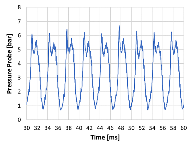
The spatially averaged .csv output includes the file probe.csv. This output is generated by the monitor probe settings discussed in the Output Controls section. If you open this file and plot the only two columns present, you will generate a graph similar to the one reported in Figure 17.5: Pressure probe during 1 revolution, and covers the entire simulation time. For the entire duration of the simulation the pressure at the probe location is recorded every 1e-6 seconds. The oscillating behavior is due to the pockets of liquid passing by the probe location.
During the simulation, the compressible flow solver predicts the locations where cavitation is likely to occur due to a sudden pressure reduction. To better show this effect, the angular velocity of the gears has been increased, and the outlet volume flow rate is reported at various RPM in Figure 17.7: Vapor volume fraction location prediction at 8000 RPM (time is in seconds). These values can be easily extracted from the Time-avg Vol Flow Rate of All Outlets within the open_boundary_flow.csv spatially averaged output. For the higher RPM, the gerotor pump behavior differs from the ideal pump, and a lower-volume flow rate is detected at the outlet.
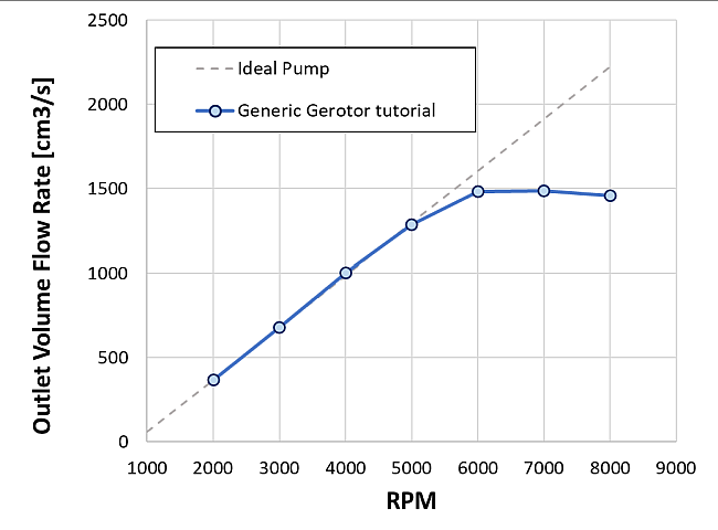
Figure 17.7: Vapor volume fraction location prediction at 8000 RPM (time is in seconds) identifies areas where cavitation occurs for the highest-RPM case, with vapor volume fraction iso-surfaces at 0.4, 0.6, and 0.8.
The following Show-Me animation is presented as an animated GIF in Forte's online documentation at the Ansys Help website. If you are reading the PDF version of this manual and want to see the animated GIF, access this section in that online documentation. The interface shown may differ slightly from that in your installed product.