This tutorial describes a nozzle flow simulation using Ansys Forte CFD. As in a typical fuel injector framework, the internal flow is driven by the high pressure-gradient between the entrance and the exit of the nozzle. The working fluid is water, and the Eulerian two-phase flow solver is employed. Refer to the Forte Theory Manual (available at the Ansys Help website) to learn more about the governing equations.
The following sections describe the provided files, time required, prerequisites, and a method for comparing your generated project file (.ftsim) with the one provided in the tutorial download.
This tutorial covers all the set-up steps, but Ansys recommends that you work through the Forte Quick Start Guide first (available at the Ansys Help site) and become familiar with the workflow of the Ansys Forte user interface.
The files for this tutorial are obtained by downloading the
nozzle_flow_tutorial.zip file
here
.
Note: For 2024 R1, the project file set-up has been updated from previous releases. The previous release, 2022 R1, requires a release-specific download of the tutorial files from the Forte 2022 R1 page at the Ansys Help website.
Unzip nozzle_flow_tutorial.zip to your working folder.
The only file provided for this tutorial is the Forte project file, a fully configured project file. It is named:
Nozzle_Flow_Tutorial.ftsim: The fully configured Forte project file.
The tutorial sample compressed archive is provided as a download. You have the opportunity to select the location for the file when you download and uncompress the sample files.
Note: This tutorial is based on a fully configured sample project that contains the tutorial project settings. The description provided here covers the key points of the project set-up but is not intended to explain every parameter setting in the project. The project files have all custom and default parameters already configured; the text highlights only the significant points of the tutorial.
Forte may be launched in a command line mode to perform certain tasks such as preparing a run for execution, importing project settings from a text file, or various other tasks described in the Forte User's Guide. One of these tools allows exporting a textual representation of the project data to a text file.
Example
forte.sh CLI -project <project_name>.ftsim -export tutorial_settings.txt
Briefly, you can double-check project settings by saving your project and then running the command-line utility to export the settings in your tutorial project (<project_name>.ftsim), and then use the command a second time to export the settings in the provided final version of the tutorial. Compare them with your favorite diff tool, such as DIFFzilla. If all the parameters are in agreement, you have set up the project successfully. If there are differences, you can go back into the tutorial set-up, re-read the tutorial instructions, and change the setting of interest.
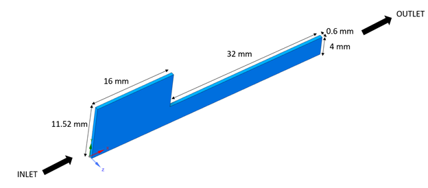
The problem considers a simple nozzle geometry, as shown in Figure 19.1: Nozzle geometry. The problem is reduced to a 2-D planar approximation that is extruded by 0.6 mm in the z-direction. The inlet/outlet diameter ratio is kept at 2.88, with an outlet orifice radius of 4 mm. The flow enters the domain from the left at 5 bar and exits on the right side at a pressure slightly smaller than atmospheric. The nozzle presents a sudden section reduction, 16 mm towards the outlet from the entrance, and because of this sharp edge, the flow separates from the wall. The working fluid is water.
The project setup workflow follows the top-down order of the workflow tree in the Ansys Forte Simulate interface. The components irrelevant to the present project will not be mentioned in this document, and you can simply skip them and use the default model options.
Note: Changed values on any Editor panel do not take effect until you press the Apply button. Always press the Apply button after modifying a value, before moving to a new panel or the Workflow tree.
The geometry used in this tutorial is basically a 2-D nozzle section extruded by 0.6 mm in the z direction. The geometry file in the .tgf format is not provided separately as with the other Forte tutorials, but it is already included in the .ftsim project file. Users can recreate the .tgf geometry file and import it through the Geometry node in the Forte project. If you do so, don’t forget to create a single volume watertight geometry and to label the surfaces to facilitate the following setup steps. In a simple geometry like this one, Ansys recommends avoiding over-refining the surface mesh.
Automatic mesh generation in Forte requires you to specify a material point, a global mesh size that serves as the reference size for mesh refinement, and various refinement controls. In this tutorial the Material Point is placed ½ unit cell length away from any boundaries. Specifically at:
X = 0.15 cm
Y = 0.15 cm
Z = 0.15 cm
Set the Global Mesh Size to 0.3 mm. Then add two Surface Refinement Depth features: one named OpenBoundaries applied to the inlet and outlet surfaces, and the other one named Walls, applied to the wall surfaces. To both, a refinement of 1/2 of the global mesh size extending for 1 cell layer is applied.
Tip: Locating the Material Point outside of the fluid domain is a commonly encountered set-up error that causes meshing failure. Be sure to set the material point inside the fluid domain.
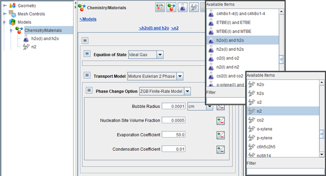
The working fluid in this nozzle tutorial is water. To set it up, go to the
Chemistry/Materials node, click the New Liquid and Vapor
Pair icon ![]() and select the pair h2o(l) and h20 as shown in
Figure 19.2: Liquid and gas properties panels. Once you have
selected your working fluid, you can either use the Forte library liquid properties, or
Override the Database Liquid Density and Viscosity
with Constant Values. Similarly, click the New Gas
Species icon
and select the pair h2o(l) and h20 as shown in
Figure 19.2: Liquid and gas properties panels. Once you have
selected your working fluid, you can either use the Forte library liquid properties, or
Override the Database Liquid Density and Viscosity
with Constant Values. Similarly, click the New Gas
Species icon ![]() and select n2. Note that adding n2 is not required
for this tutorial, you could simply have water vapor as phase 1 in Figure 19.2: Liquid and gas properties panels. Liquid and gas properties panels.
Nevertheless, it is included to show you how to create your own mixture composition.
and select n2. Note that adding n2 is not required
for this tutorial, you could simply have water vapor as phase 1 in Figure 19.2: Liquid and gas properties panels. Liquid and gas properties panels.
Nevertheless, it is included to show you how to create your own mixture composition.
In the same Chemistry/Materials node, keep the default Ideal Gas option for the Equation of State, select Mixture Eulerian 2 Phase for the Transport Model option and set the Phase Change Option to ZGB Finite-Rate Model. Keep the default parameter values and click Apply.
This tutorial uses the RANS RNG k-epsilon turbulence model, which is the default turbulence model option. Other turbulence modeling options are available under Models > Transport > Turbulence.
Boundary conditions must be specified for each of the surfaces found in the Geometry node. To match the provided project, follow these instructions for each boundary condition:
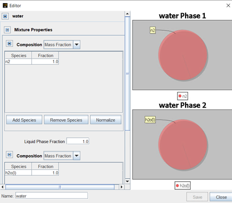
Inlet: Defined as an inlet boundary ![]() . In the Composition option, Create a new
multiphase mixture. A window will be displaced and will allow you to specify your
mixture composition. Set it as shown in
Figure 19.3: Set up water as working fluid. and be sure to set the Liquid
Phase Fraction to be 1. Save it and apply it to the inlet
composition. Pick the inlet surface as the selected
Location where this boundary condition will apply, set the
Static Pressure to 5e5 Pa, leave
the Turbulent Kinetic Energy to 0.4 m2/sec2, the
Turbulence Eddy Dissipation Rate to
7e4 m2/sec3, and finally set the Static
Temperature to 300 K.
. In the Composition option, Create a new
multiphase mixture. A window will be displaced and will allow you to specify your
mixture composition. Set it as shown in
Figure 19.3: Set up water as working fluid. and be sure to set the Liquid
Phase Fraction to be 1. Save it and apply it to the inlet
composition. Pick the inlet surface as the selected
Location where this boundary condition will apply, set the
Static Pressure to 5e5 Pa, leave
the Turbulent Kinetic Energy to 0.4 m2/sec2, the
Turbulence Eddy Dissipation Rate to
7e4 m2/sec3, and finally set the Static
Temperature to 300 K.
Outlet: Defined as an inlet boundary ![]() , to force the reverse flow condition to be explicitly defined. After
selecting the outlet surface as Location, set the
Static Pressure to 9.5e4 Pa and
the Turbulent Kinetic Energy and Dissipation Rate
to 1 m2/sec2 and
1 m2/sec3, respectively. Keep the Static
Temperature at 300 K.
, to force the reverse flow condition to be explicitly defined. After
selecting the outlet surface as Location, set the
Static Pressure to 9.5e4 Pa and
the Turbulent Kinetic Energy and Dissipation Rate
to 1 m2/sec2 and
1 m2/sec3, respectively. Keep the Static
Temperature at 300 K.
Walls: Defined as a wall boundary ![]() . Select the surface named walls as
Location, apply the Law of the Wall as a
Wall Slip Condition. Leave the rest of the editor panel at default
values and disable the Heat Transfer check box.
. Select the surface named walls as
Location, apply the Law of the Wall as a
Wall Slip Condition. Leave the rest of the editor panel at default
values and disable the Heat Transfer check box.
FrontBack: Defined as a wall boundary ![]() . Similar to the previous boundary condition, select the
front and back surfaces as
Location, but this time allow the Wall Slip
Condition to be Free Slip.
. Similar to the previous boundary condition, select the
front and back surfaces as
Location, but this time allow the Wall Slip
Condition to be Free Slip.
Symmetry: Defined as a dymmetry boundary  . Select the bottom surface.
In the Initial Conditions under Default Initialization, use the same composition shown in Figure 19.3: Set up water as working fluid. Set the Temperature to 300 K, the Pressure to 4.5e5 Pa, the Turbulent Kinetic Energy and Dissipation Rate to 0.4 m2/sec2 and 7e4 m2/sec3, respectively, and finally, the Velocity in the X-direction to 10 m/sec.
Let the simulation be Time Based and enter the Max. Simulation Time of 20 msec. Leave everything else as default.
In the Time Step editor panel, set the Initial Simulation Time Step to be 1e-6 sec, and the Max. Simulation Time Step to be 1e-4 sec. Then, in the Advanced Time Step Control Options, double both the Fluid Acceleration Factor and the Rate of Strain Factor.
In the Chemistry Solver editor panel, turn off chemistry by setting Activate Chemistry to Always Off.
For the Transport Terms controls, Ansys recommends using 1e-5 as the Pressure Iteration Tolerance and increasing to 100 the SIMPLE Iteration Threshold for Limiting Time Step. These settings are suggested when either liquids or 2-phase flows are involved in the simulation.
Output controls determine what data are stored for viewing during the simulation and for creating plots, graphs, and animations in Ansys EnSight.
Spatially Averaged and Spray: Select Time in the Spatially Averaged Output Control and set the interval to 1e-6 sec, then choose the species of interest, if any.
Restart Data: It is good practice to enable the restart data writing at the end of a simulation in case you want continue it later. You could also choose to have restart files written at a certain frequency or at specified times, depending on your needs.
Additional Output: Starting with Ansys Forte 2022
R1, alongside the standard spatially resolved outputs
(.ftres format), Forte offers the possibility to have an
additional or an alternative set of output format, namely EnSight DVS
(Dynamic Visualization Store). The DVS format helps reduce the loading time and the stepping
through transient solution points in Ansys EnSight, thanks to the smaller size of the files
generated. Better performance is also expected during the solution writing, especially when
running a job on a cluster with many processors. To utilize the EnSight DVS format, start
by clicking the EnSight ![]() icon on the Additional Output editor panel. Then check the
Enabled box under EnSight DVS Settings. The
output settings follow the same structure as Forte's native spatially resolved outputs.
In other words, select your Interval Based Output Control frequency and
pick your Solution Variables of interest. Only those in this list will
be found in EnSight, so it is always suggested to have amongst this at least Pressure and
Velocity Magnitude. If you scroll down in the same EnSight DVS editor
panel you can also add the Spatially Averaged Datasets in the same
additional output files set.
icon on the Additional Output editor panel. Then check the
Enabled box under EnSight DVS Settings. The
output settings follow the same structure as Forte's native spatially resolved outputs.
In other words, select your Interval Based Output Control frequency and
pick your Solution Variables of interest. Only those in this list will
be found in EnSight, so it is always suggested to have amongst this at least Pressure and
Velocity Magnitude. If you scroll down in the same EnSight DVS editor
panel you can also add the Spatially Averaged Datasets in the same
additional output files set.
Note: If you miss selecting the Enabled box, no EnSight DVS output will be generated, even if the rest of the panel is properly set. DVS output can be enabled independently from Forte's spatially resolved output. Therefore it often makes sense to disable Forte's spatially resolved output when using DVS.
The DVS results will be contained in a subfolder of the run directory, named according to the user-supplied name of the DVS output added to the Workflow tree. To load the results in EnSight, within an EnSight session, choose File > Open and select the .dvs file from this directory or use the EnSight launcher shortcut on Forte's Run panel, which will search for and provide a list of available .dvs files in the analysis directory that can be preselected and passed to the newly launched EnSight instance.
To detect potential problems due to surface intersection or mesh generation before the
simulation is started, navigate to the Preview Simulation node. On the
Mesh Generation panel, set the Time Option to
Time for investigating a specific Time or to
Time Range for a more extensive investigation, then select
Check for Surface Intersections and/or Include Volume
Mesh (highly recommended for a case with moving parts), and finally launch the
preview by clicking the Generate Mesh
![]() icon. Due to the nature of this tutorial, it is a good idea to create a
mesh preview with multiple steps spanning over an entire revolution to check the mesh quality.
Nevertheless, the feature can be used to make sure all the other parts behave as expected and
the volume mesh generation is appropriate.
icon. Due to the nature of this tutorial, it is a good idea to create a
mesh preview with multiple steps spanning over an entire revolution to check the mesh quality.
Nevertheless, the feature can be used to make sure all the other parts behave as expected and
the volume mesh generation is appropriate.
The run settings depend on the system and environment for your simulations. Change the number of cores to use for this simulation according to the resources available to you by navigating to Run Settings > Run Options, and under Job Script Options, setting the number of cores for Default MPI Arguments. No other changes are needed and you can continue launching the simulation.
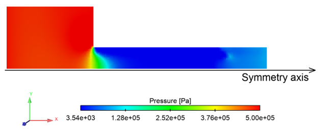
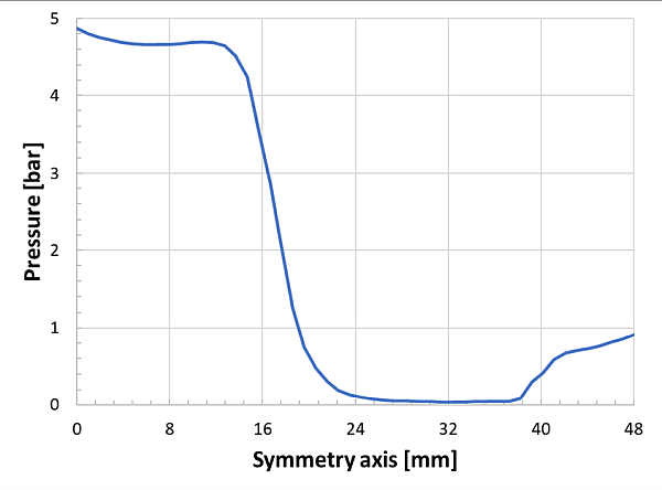
The final section of this tutorial is a collection of the results at 20 ms when the flow has basically reached its steady state. In Figure 19.4: Pressure distribution on the z-middle plane at 20 ms, the pressure distribution is shown. The flow entering the domain at 5 bar is then forced to cross the portion of the nozzle with the reduced diameter. The cross-section is suddenly reduced, and we assign a halving of the pressure. The pressure remains constant until the flow is close to the exit where the higher back-flow pressure is imposed. To better understand how the pressure develops along the axial direction of the flow, see Figure 19.5: Pressure evolution along the symmetry axis. Here the pressure is extracted at the symmetry axis, and you can see more clearly that the pressure drop occurs at 16 mm from the entrance simultaneously with the orifice diameter reduction.
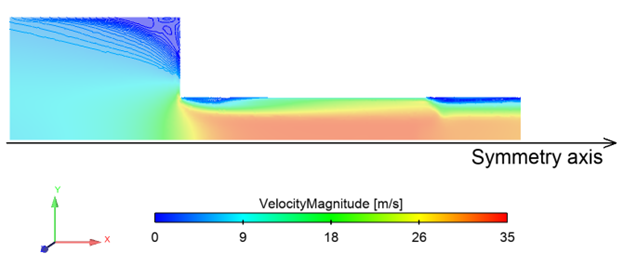
Similarly, in Figure 19.6: Velocity magnitude distribution on the z-middle plane at 20 ms, with recirculation zones and Figure 19.7: Velocity magnitude evolution along the symmetry axis at 20 ms the velocity magnitude distribution and its profile along the symmetry axis are depicted. In the spatial velocity results, the velocity field is made transparent so that you can notice 3 recirculation zones. The first one is in the larger diameter section on its top right side, where the flow is forced to curve downwards. The second one the point when, due to the flow separation, a flow portion remained trapped after the section restriction at the orifice. The third one is close to the exit, where the backflow with a higher pressure is trying to reenter the domain. These 3 recirculation zones are identified by opaque contour lines displayed in Figure 19.6: Velocity magnitude distribution on the z-middle plane at 20 ms, with recirculation zones.
Figure 19.6: Velocity magnitude distribution on the z-middle plane at 20 ms, with recirculation zones
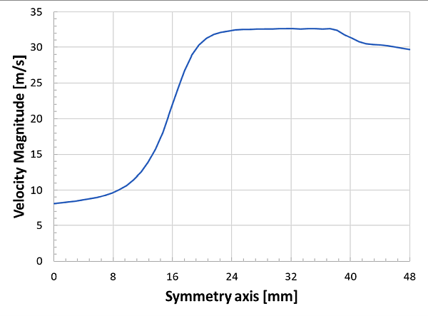
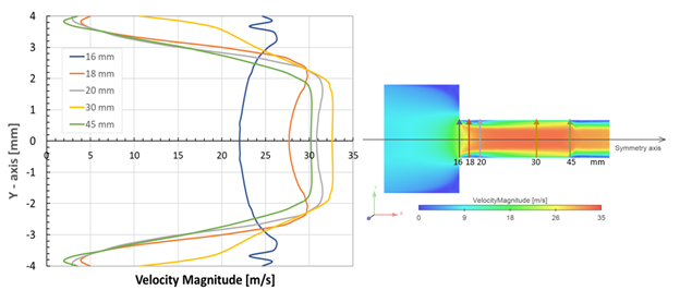
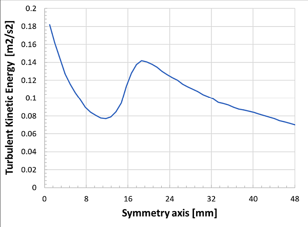
To follow the evolution of the flow, the velocity magnitude is extracted at 16, 18, 20, 30, and 45 mm from the inlet and plotted it against the y-axis, as shown in Figure 19.8: Left: velocity magnitude profiles at various distances from the entrance; Right: velocity magnitude contour at the z-middle plane at 20 ms (results are mirrored with respect to the symmetry axis for clearer understanding). For a better understanding, the results have been extended and mirrored over the negative y-axis values, but keep in mind that only the domain above the symmetry axis has been simulated. You can see how at the entrance of the smaller section (at 16 mm) the flow starts to accelerate from the sides and gets to about 22 m/s at the center. By proceeding forward, the flow keeps accelerating, orange and gray lines, until approximately 33 m/s, becoming fully developed at about 30 mm, yellow line. Right before the flow exit at 45 mm, the velocity is reduced to about 28 m/s. The turbulent kinetic energy along the symmetry line is plotted in Figure 19.9: Turbulent kinetic energy along the symmetry axis at 20 ms.
Figure 19.8: Left: velocity magnitude profiles at various distances from the entrance; Right: velocity magnitude contour at the z-middle plane at 20 ms (results are mirrored with respect to the symmetry axis for clearer understanding)
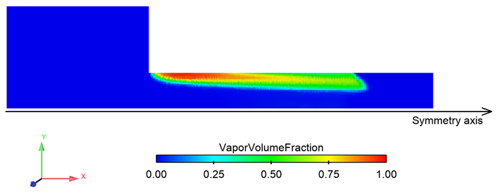
When the nozzle channel shrinks at 16 mm, the pressure drops, the flow accelerates, and cavitation effects can be observed. Examine the vapor volume fraction in Figure 19.10: Vapor volume fraction distribution on the z-middle plane at 20 ms.