This tutorial describes how to use Ansys Forte CFD to simulate the gas flow in a scroll compressor. Scroll compressors are positive displacement compressors usually employed in air conditioning, refrigeration, and heat pump applications.
This document will go through all the simulation setup steps, with emphasis on the following aspects that are unique or important to scroll compressors:
Requirements for surface geometry preparation
Small gap handling using gap refinement controls and gap model
Setup of orbiting motion, which is a special case of planetary motion
Simulation preview for checking boundary motion and potential surface intersection
Visualization of simulation results
The following sections describe the provided files, time required, and prerequisites.
This tutorial will cover all the setup steps, but we recommend that you work through the Forte Quick Start Guide first and become familiar with the workflow of the Ansys Forte user interface.
The files for this tutorial are obtained by downloading the
scroll_compressor.zip file
here
.
Unzip scroll_compressor.zip to your working folder.
Files provided in this tutorial include a Forte project file that has been fully configured as well as the surface geometry input files that can be used to set up the Forte project from scratch. Specifically, the files include:
Scroll_Compressor_Tutorial.ftsim: The fully configured Forte project file.
Scroll_Compressor_Surface_Geometry.tgf: Surface geometry input file in Ansys Fluent Meshing faceted geometry (.tgf) format, which was exported from Ansys SpaceClaim.
The tutorial sample compressed archive is provided as a download. You have the opportunity to select the location for the file when you download and uncompress the sample files.
Note: This tutorial is based on a fully configured sample project that contains the tutorial project settings. The description provided here covers the key points of the project setup but is not intended to explain every parameter setting in the project. The project files have all custom and default parameters already configured; the text highlights only the significant points of the tutorial.
Forte may be launched in a command line mode to perform certain tasks such as preparing a run for execution, importing project settings from a text file, or various other tasks described in the Forte User's Guide. One of these tools allows exporting a textual representation of the project data to a text file.
Example
forte.sh CLI -project <project_name>.ftsim -export tutorial_settings.txt
Briefly, you can double-check project settings by saving your project and then running the command-line utility to export the settings in your tutorial project (<project_name>.ftsim), and then use the command a second time to export the settings in the provided final version of the tutorial. Compare them with your favorite diff tool, such as DIFFzilla. If all the parameters are in agreement, you have set up the project successfully. If there are differences, you can go back into the tutorial set-up, re-read the tutorial instructions, and change the setting of interest.
The geometry and working principle of the sample scroll compressor are illustrated in Figure 15.1: Configuration of the example scroll compressor. In a scroll compressor, gaseous refrigerant is admitted in the periphery and discharged in the central region of a mechanical compressing assembly. This assembly is formed by two identical spiral-shaped scrolls (one fixed scroll and one orbiting scroll) and a casing that encloses these two scrolls. The orbiting motion of the orbiting scroll initiates gas pockets formed between the two scrolls at the periphery of the assembly and migrates the pockets to the central region of the assembly. During this migration, the volume of the gas pockets is continuously reduced, resulting in an increase in both the pressure and temperature of the gas. The compressed gas is eventually discharged when the pockets are exposed to the discharge port. The dimension and operating condition specifications are listed in Table 15.1: Dimensions and operating conditions of the example scroll compressor.
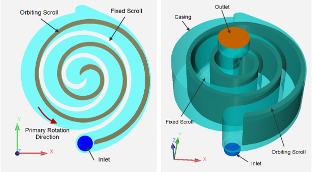
Table 15.1: Dimensions and operating conditions of the example scroll compressor
| Item | Value | Units |
|---|---|---|
| Casing diameter | ~14 | cm |
| Scroll height | ~5 | cm |
| Eccentric radius | 0.785 | cm |
| Working fluid | R-410A (50% R32 + 50% R125 by vol.) | |
| Suction pressure (Total) | 9.978 | bar |
| Suction temperature (Total) | 293 | K |
| Discharge pressure (Total) | 33.853 | bar |
| Discharge temperature (Total) | 373 | K |
| Rotation Speed | 3000 | rev/min |
The project setup workflow follows the top-down order of the Workflow tree in the Ansys Forte Simulate interface. For the configuration components not mentioned in this tutorial, you can simply skip them and use the default model options
This simulation uses Forte's on-the-fly automatic mesh generation (AMG) feature, which only requires the bounding surface geometry as an input and does not involve volume mesh generation ahead of the calculation. The surface geometry to be imported into Forte is in Fluent Meshing faceted geometry (.tgf) format, which was exported from the solid geometry created in SpaceClaim. Although the TGF format is used in this tutorial, several other formats are also allowed. See the Geometry Import section in the Forte User's Guide for details.
Since the scroll and casing geometries involve curved surfaces in 3-D and there are tiny gaps between the side surfaces of scroll and casing, the curved surfaces are required to be sufficiently smooth in order to avoid surface intersection during the rotation. When exporting the TGF file from SpaceClaim, we recommend that you choose the Fine option for the Facet Resolution of the TGF file. The Angle resolution should not be much larger than 4°.
Now let us import the surface geometry into the Forte Simulate user interface. Open
the Geometry panel, click the Import Geometry ![]() icon, select Surfaces from TGF file as the import
option, and select the provided TGF file,
Scroll_Compressor_Surface_Geometry.tgf. Ensure that the
Invert Normals box is checked and accept all other default options on
the Import Options wizard window.
icon, select Surfaces from TGF file as the import
option, and select the provided TGF file,
Scroll_Compressor_Surface_Geometry.tgf. Ensure that the
Invert Normals box is checked and accept all other default options on
the Import Options wizard window.
The fluid domain in this case is formed by two watertight surface groups, which are the bounding surfaces of the two solids in SpaceClaim. The first group consists of “inlet”, “outlet”, “intake-port”, “discharge-port”, “static-scroll-end”, and “static-scroll-side”; the second group includes the two surfaces that form the orbiting scroll: “orbiting-scroll-end” and “orbiting-scroll-side”. Forte requires that the end surfaces of the orbiting scrolls be put inside the casing and away from the casing’s end surfaces by a tiny tolerance. In the provided geometry file, this tiny tolerance is 1 µm. By default, the gap between the orbiting scroll end surface and the casing end surface will not be meshed in the volume mesh. However, if the end gap sizes are physically large enough and it is desirable to model the flow leakage through them, we can force these gaps to be meshed by using the gap refinement controls that will be discussed later in Automatic Mesh Generation Setup.
In Forte, the normal vectors of the triangulated surface mesh are required to point towards the exterior of the fluid domain. In the .tgf file, the normal vectors point to the interior of the two watertight surface groups. When the .tgf geometry is imported, all the normal vectors are inverted. As a result, the surface normals of the orbiting scroll surfaces should be inverted again such that they point to the exterior of the fluid domain. To do so, multi-select (hold Ctrl and click) surfaces “orbiting-scroll-end” and “orbiting-scroll-side” on the Geometry node of the Workflow tree, and on the right-click menu, choose Invert Normals. You can double-check the normals of a surface by turning on Normals using the right-click menu.
Forte's automatic mesh generation requires you to specify a material point, a global mesh size that serves as the reference size for mesh refinement, and various refinement controls.
Material Point: The Material Point ![]() should always lie inside the fluid domain throughout the simulation and
should be located at least one unit cell length away from any boundaries. In this tutorial
case, we choose to put the material point inside the discharge port: X = 0.0 cm, Y
= 13.5 cm, Z = 30.0 cm.
should always lie inside the fluid domain throughout the simulation and
should be located at least one unit cell length away from any boundaries. In this tutorial
case, we choose to put the material point inside the discharge port: X = 0.0 cm, Y
= 13.5 cm, Z = 30.0 cm.
Global Mesh Size: Set the Global Mesh Size to 0.2 cm.
Three types of refinement controls are used in this tutorial: Surface
Refinement Depth ![]() , SAM (Solution Adaptive Mesh)
, SAM (Solution Adaptive Mesh) ![]() , and Gap Feature Control
, and Gap Feature Control
![]() . Detailed mesh control parameters are listed in Table 15.2: Settings for Mesh Control refinements. The Active property is
set to Always for all the mesh controls. For the Gap Feature
Control, the Surface Proximity is set to 0.15
cm, and Enable Gap Model is turned ON.
. Detailed mesh control parameters are listed in Table 15.2: Settings for Mesh Control refinements. The Active property is
set to Always for all the mesh controls. For the Gap Feature
Control, the Surface Proximity is set to 0.15
cm, and Enable Gap Model is turned ON.
Table 15.2: Settings for Mesh Control refinements
| Item | Refinement type | Refinement location | Refinement level | Refinement layers |
|---|---|---|---|---|
| Open_Boundaries | Surface | inlet, outlet | 1/2 | 1 |
| Static_Walls | Surface | discharge-port, intake-port, static-scroll-end, static-scroll-side | 1/2 | 1 |
| Orbiting_Scroll_Side | Surface | orbiting-scroll-side | 1/2 | 1 |
| Orbiting_Scroll_Ends | Surface | orbiting-scroll-end | 1/4 | 1 |
| SAM_Velocity_Grad | SAM Quantity Type = Gradient of Solution Field; Solution Variables = VelocityMagnitude; Bounds = Statistical; Sigma Threshold = 0.5 | Entire Domain | 1/2 | |
| Gaps | Gap feature | (orbiting_scroll_side, static_scroll_side) | 1/4 |
The Gap Feature Control
![]() is a mesh refinement control that is especially useful for handling the
small gaps in compressors. This control automatically detects small gaps between the
specified surface pair based on the user-specified Surface Proximity
criterion and applies refinement in the detected gap region based on the user-specified
refinement level. When Gap Feature Control is used, the spatially
resolved solution will contain a variable called GapCellFlag, which uses non-zero integer
values to mark the zones identified as gap zones.
is a mesh refinement control that is especially useful for handling the
small gaps in compressors. This control automatically detects small gaps between the
specified surface pair based on the user-specified Surface Proximity
criterion and applies refinement in the detected gap region based on the user-specified
refinement level. When Gap Feature Control is used, the spatially
resolved solution will contain a variable called GapCellFlag, which uses non-zero integer
values to mark the zones identified as gap zones.
Forte does not require the gap zones to be finely resolved using tiny CFD cells. In this tutorial, the Cartesian cell size in the gap zone is 0.05 cm, which means that some of the gaps only contain a fraction of a Cartesian cell cut by the physical boundary. To compensate for the under-resolution in the gap zones, the Gap Model is used to apply a momentum sink term, which accounts for the underpredicted wall shear stress and over-predicted mass flow rate on the coarse grid. The Gap Model takes both the gap size and the local fluid cell size as inputs, and therefore the flow solution is not expected to be very sensitive to the gap refinement level.
The Gap Size Scale Factor can be used to enlarge or shrink the gap sizes measured on the geometry. The scaled gap size is then used as the input for the gap model in each local CFD cell in the gap zone. If the gap size in the geometry accurately reflects the size in the actual compressor, the best practice is to use the default value of 1.0. In this sample scroll compressor case, the smallest gap size is about two times of that in the actual compressor, therefore the gap size scale factor is set to 0.5 to reduce flow leakage through gaps in the simulation. When using simulation to guide compressor design, this gap size scale factor also allows you to study the impact of gap size on simulation results without the need of modifying the geometry itself.
As mentioned earlier, there is a 1 µm distance tolerance between the end surface of
the orbiting scroll and the end surface of the casing (the surface is called
“static-scroll-end”) on both ends. Forte will ignore this tiny gap by
default. However, if the end gaps are large enough and it is of interest to model the flow
leakage through them, you can use the Gap Feature Control
![]() to mesh these gaps.
to mesh these gaps.
In Forte, a chemistry set in Chemkin format is used to define the properties of the
working fluid. This scroll compressor is for refrigeration applications. The working fluid
is R-410A, which is a mixture of R32 and R125. It will be modeled using the real gas model.
Ansys Forte supplies a chemistry set for various refrigerants, called
Refrigerants.cks, which is stored in the data folder of your Forte
installation. To import this chemistry set, go to the Workflow tree and under
Models > Chemistry/Materials, click
New Import Chemistry ![]() and select Refrigerants.cks in the data folder of
the Forte installation. This chemistry set contains R32 and R125 as species. To create
the R-410A mixture, click the Mixture
and select Refrigerants.cks in the data folder of
the Forte installation. This chemistry set contains R32 and R125 as species. To create
the R-410A mixture, click the Mixture ![]() icon on the menu bar, select the Create new...
option under gas_mixtures, and click the Pencil
icon on the menu bar, select the Create new...
option under gas_mixtures, and click the Pencil![]() icon. In the pop-up Mixture Editor window, click Add Species
to add R32 and R125 and set both of
their Mole Fractions to 0.5. To turn on the real
gas model option, choose Real Gas as the Equation of
State option on the Models >
Chemistry/Materials panel.
icon. In the pop-up Mixture Editor window, click Add Species
to add R32 and R125 and set both of
their Mole Fractions to 0.5. To turn on the real
gas model option, choose Real Gas as the Equation of
State option on the Models >
Chemistry/Materials panel.
This tutorial uses the RANS RNG k-ε turbulence model, which is the default turbulence model option. Other turbulence modeling options are available under Models > Transport > Turbulence, such as LES models.
Use the icons on the Boundary Conditions panel to add new boundary conditions. The boundary conditions used in this project are explained below:
Inlet: Defined as an inlet boundary ![]() . For Composition on the inlet setup panel, select
the R-410A mixture created earlier. Select surface
inlet as the Location. Choose the
Total Pressure option for Inlet type and set the
pressure to 9.978 bar. Keep the default turbulence parameters for the
inflow. Choose Total Temperature as the Temperature
Option and set the temperature to 293 K.
. For Composition on the inlet setup panel, select
the R-410A mixture created earlier. Select surface
inlet as the Location. Choose the
Total Pressure option for Inlet type and set the
pressure to 9.978 bar. Keep the default turbulence parameters for the
inflow. Choose Total Temperature as the Temperature
Option and set the temperature to 293 K.
Discharge: The discharge outlet should be defined as an inlet
boundary ![]() as well because we need the reverse flow condition to be explicitly
defined. For Composition, select the same R-410A
mixture. Select surface outlet as the Location.
Choose the Total Pressure option for Inlet type
and set the pressure to 33.853 bar. Keep the default turbulence
parameters for the inflow. Choose Total Temperature as the
Temperature Option and set the temperature to 373
K.
as well because we need the reverse flow condition to be explicitly
defined. For Composition, select the same R-410A
mixture. Select surface outlet as the Location.
Choose the Total Pressure option for Inlet type
and set the pressure to 33.853 bar. Keep the default turbulence
parameters for the inflow. Choose Total Temperature as the
Temperature Option and set the temperature to 373
K.
Static-walls: Defined as a wall boundary ![]() . This boundary condition includes all static walls in this sample, but
you can choose to split it into multiple wall boundaries if needed. Select surface
intake_port, discharge_port,
static_scroll_end, and static_scroll_side as the
Location. Turn ON Heat Transfer and set
Wall Temperature to 333.0 K.
. This boundary condition includes all static walls in this sample, but
you can choose to split it into multiple wall boundaries if needed. Select surface
intake_port, discharge_port,
static_scroll_end, and static_scroll_side as the
Location. Turn ON Heat Transfer and set
Wall Temperature to 333.0 K.
Orbiting-scroll-wall: Defined as a wall boundary ![]() . Select surfaces orbiting-scroll-end and
orbiting-scroll-side as the Location. Turn off
Heat Transfer to model this wall as adiabatic. Turn on Wall
Motion and set Motion Type as Planetary
Motion. Both the primary axis and secondary axis require an
Origin and a Direction vector as the inputs. To
facilitate the setup, let us create two reference frames for these two axes. Go to
Geometry > Reference Frames, click the
New Reference Frame
. Select surfaces orbiting-scroll-end and
orbiting-scroll-side as the Location. Turn off
Heat Transfer to model this wall as adiabatic. Turn on Wall
Motion and set Motion Type as Planetary
Motion. Both the primary axis and secondary axis require an
Origin and a Direction vector as the inputs. To
facilitate the setup, let us create two reference frames for these two axes. Go to
Geometry > Reference Frames, click the
New Reference Frame![]() icon to create two new reference frames: primary-shaft
and secondary-shaft. For reference frame
primary-shaft, set the New Origin to (X
= 0.0 cm, Y = 13.65 cm, Z = 25.0 cm); for reference frame
secondary-shaft, set the New Origin to
(X = 0.785 cm, Y = 13.65 cm, Z = 25.0 cm). Now go back to this boundary
condition panel. By using the two reference frames for the Primary and
Secondary Axes, the Origin and
Direction of these two axes are simply the origin (X = 0.0
cm, Y = 0.0 cm, Z = 0.0 cm) and Z-axis (X = 0.0, Y = 0.0, Z =
1.0) of the corresponding reference frames. See the fully configured Forte
project for details. To create an orbiting motion, the angular velocities of the primary
rotation and secondary rotation should have the same magnitude but opposite direction.
Therefore, set Primary Angular Velocity to 3000
RPM and set Secondary Angular Velocity to -3000
RPM. Note that the rotation direction follows the right-hand rule.
icon to create two new reference frames: primary-shaft
and secondary-shaft. For reference frame
primary-shaft, set the New Origin to (X
= 0.0 cm, Y = 13.65 cm, Z = 25.0 cm); for reference frame
secondary-shaft, set the New Origin to
(X = 0.785 cm, Y = 13.65 cm, Z = 25.0 cm). Now go back to this boundary
condition panel. By using the two reference frames for the Primary and
Secondary Axes, the Origin and
Direction of these two axes are simply the origin (X = 0.0
cm, Y = 0.0 cm, Z = 0.0 cm) and Z-axis (X = 0.0, Y = 0.0, Z =
1.0) of the corresponding reference frames. See the fully configured Forte
project for details. To create an orbiting motion, the angular velocities of the primary
rotation and secondary rotation should have the same magnitude but opposite direction.
Therefore, set Primary Angular Velocity to 3000
RPM and set Secondary Angular Velocity to -3000
RPM. Note that the rotation direction follows the right-hand rule.
For Composition, select the mixture R-410A created earlier . Set Temperature to 350 K and Pressure to 9.975 bar. It is not critical to have well guessed initial conditions because the initial mixture can be quickly flushed out and overridden by steady operation conditions after 2 to 3 revolutions.
Simulation Limits: Choose the Time Based option to specify the Simulation End Point and set Max. Simulation Time to 0.1 s. This duration covers five complete revolutions for the primary shaft. (Time for each resolution can be calculated as 60/RPM s).
Time Step: Forte uses adaptive time step controls to adjust the actual time step size for each transient flow integration step. The user-specified max time step will be used if the time step is not subject to other constraints listed under Advanced Time Step Control Options. For rotating machinery simulation, the rule of thumb for choosing the Maximum Simulation Time Step is to have at least 10 time steps per degree of rotation of the fastest rotating motion in the system. Using this guideline, the Max Time Step can be estimated as 60/(RPM*360*10) = 1/(RPM*60) s, which gives 5.56E-6 s for RPM = 3000. In this tutorial, the Max Time Step is set to 5.0E-6 s. For the Advanced Time Step Control Options, typically it is acceptable to relax the Fluid Acceleration Factor and Rate of Strain Factor to achieve larger time steps without affecting the accuracy and stability very much. In this calculation, these two factors are set to 1.0 and 1.2, respectively. Both are two times their default values. It is risky to change the other control factors because relaxing them may cause the solution to become unstable.
Chemistry Solver: Set the Activate Chemistry option to Always Off because this simulation does not involve chemical reactions.
Spatially Resolved: Use Time for the Output Timing Control option. Set Interval Based Output Control to output every 0.01 s, which corresponds to a half revolution. Turn on User Defined Output Controls and create a time list to save spatially resolved solutions at locations of interest. In the fully configured .ftsim file, the solutions are saved for every 5.56E-4 s (corresponding to 10 degrees of rotation) for the third revolution. For the Spatially Resolved Species list, select R32 and R125. For the Solution Variables list, select variables of interest. The minimum variable set should include Pressure, Temperature, VelocityX, VelocityY, VelocityZ, and Velocity Magnitude.
Spatially Averaged And Spray: Choose the Time option and set the output interval to 1.0E-5 s. Select species R32 and R125 for output.
Restart Data: Make sure Write Restart File at Last Simulation Step is checked ON. This option allows a restart file to be saved at the end of the current simulation. Such a restart file is useful if you decide to extend the simulation duration to do parameter studies because it provides a much better guess for initial condition than a uniform one. This practice may help save CPU time spent in simulating the initial transient process. Turn ON Interval Based Restart and set the Time Steps between Restart Writing to 500. This type of restart file can help provide a recovery point if a long-running job was unexpectedly interrupted.
Monitor Probes: On the Monitor Probes setup panel, for the
Inquiry Frequency, choose Time as the
Frequency Option and set the interval to 1.0E-5 s.
Click the New Probe icon ![]() to add new monitor probes. In this tutorial, we will add three
Geometric-based probes at different locations and one
Boundary-Condition-based probe using the
Discharge boundary.
to add new monitor probes. In this tutorial, we will add three
Geometric-based probes at different locations and one
Boundary-Condition-based probe using the
Discharge boundary.
The Geometric-based probes are called Probe_High_Pres, Probe_Medium_Pres, Probe_Low_Pres. For each of them, set Monitor Type to Geometric, choose Spherical as Geometry Shape, use the primary-shaft reference frame for the Location and set the Location to (X = 1.5 cm, Y = 0.0 cm, Z = 0.0 cm), (X = 4.0 cm, Y = 0.0 cm, Z = 0.0 cm), and (X = 6.5 cm, Y = 0.0 cm, Z = 0.0 cm), respectively, and set the Radius of the sphere to 0.2 cm. These three probes are only examples. You can customize the locations in your specific application. Select Pressure and Temperature from the Solution Variables list to monitor their local variation at the probed locations.
The Boundary-Condition-based probe is called Probe_Outlet. For this one, set Monitor Type to Boundary Condition, select the Discharge boundary from the list, and also select Pressure and Temperature from the Solution Variables list to monitor the pressure and temperature averaged over all the fluid cells adjacent to the Discharge boundary.
The Preview Simulation utility is a useful tool for checking boundary
motion, detecting potential surface intersection and verifying volume mesh generation ahead of
the calculation. Open the Mesh Generation panel under Preview
Simulation, select Time Range as the Time Option,
set the Start, End, and Step to
0.0 s, 0.02 s, 0.001 s, respectively. Since one complete revolution takes
0.02 s at 3000 RPM, this preview schedule will produce 20 snapshots within a revolution. Click
the Generate Mesh icon ![]() on the panel, then select PreviewData.dvs and click
OK on the pop-up window that appears. Ansys EnSight will be launched
automatically and the preview solutions will be gradually loaded in EnSight as soon as they
are created.
on the panel, then select PreviewData.dvs and click
OK on the pop-up window that appears. Ansys EnSight will be launched
automatically and the preview solutions will be gradually loaded in EnSight as soon as they
are created.
By default, the Check for Surface Intersections and Include Volume Mesh boxes are not selected, and the preview is only for checking surface mesh motion. This type of preview is very fast to process. You can run this preview in serial mode and create dozens of snapshots. The preview solution should come out almost instantly in EnSight.
If Check for Surface Intersections is turned ON, the preview requires slightly longer CPU time. A new Part called intersections will be added to the part list in EnSight. If any surface intersection occurs, the surface triangles involved in the intersections will show up in this new Part.
If Include Volume Mesh is turned ON, the volume mesh preview results will take considerably longer CPU time to produce. We recommend running the volume mesh preview in MPI mode and limiting the preview locations to a few snapshots. Doing snapshot check for volume mesh is valuable for detecting setup errors in material point, surface normal and also for verifying mesh refinement settings.
The run settings depend on the system and environment for your simulations. All the default options are appropriate for running this tutorial. The only thing to customize is the number of MPI processes used to run the job. The default value is 16, but it can be modified under Run Settings > Run Options > Job Script Options > Default MPI Arguments. The actual value used in the run can be further modified on the Run Simulation panel, shown as MPI Arguments. The CPU time needed to run this case is described in Time Estimate. If possible, use more MPI cores to shorten the turnaround time. Refer to the Forte User's Guide if you need to set up multiple runs in a parameter study.
This section discusses using the output to visualize and post-process results:
The spatially averaged solutions are reported in CSV format in the Run folder (Nominal).
Ansys Forte Monitor ![]() is a convenient tool for displaying these averaged solutions. Launch
Forte Monitor and open the .analysis directory of the Forte project to load the CSV
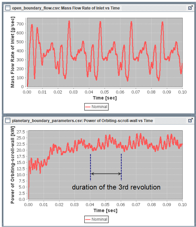
files. Several line plot examples are shown in Figure 15.2: Line plots created in Forte Monitor. The parameters plotted include mass flow rate at the Inlet
(open_boundary_flow.csv) and power of the orbiting scroll applied on
the fluid (planetary_boundary_parameters.csv). In this example, the
curves show that the simulation has largely reached a steady operation starting from the
third revolution. The cyclic pattern started to repeat for each revolution
thereafter.
is a convenient tool for displaying these averaged solutions. Launch
Forte Monitor and open the .analysis directory of the Forte project to load the CSV
files. Several line plot examples are shown in Figure 15.2: Line plots created in Forte Monitor. The parameters plotted include mass flow rate at the Inlet
(open_boundary_flow.csv) and power of the orbiting scroll applied on
the fluid (planetary_boundary_parameters.csv). In this example, the
curves show that the simulation has largely reached a steady operation starting from the
third revolution. The cyclic pattern started to repeat for each revolution
thereafter.
Ansys EnSight is the preferred tool for visualizing the spatially resolved solutions. Launch EnSight and open the .ftind file to load the solutions. The .ftind file is a solution index file, which contains the records pointing to a group of .ftres files. The actual solution data are contained in the .ftres files. If you need to control which .ftres solution(s) to load in EnSight, you can truncate or concatenate the records contained in the .ftind files in a text editor. Refer to the Forte User's Guide for details.
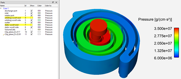
It is worth noting that the end gaps between the orbiting end surfaces (surface “orbiting-scroll-end”) and the casing end surfaces (surface “static-scroll-end”) are not meshed using fluid cells in the current setup. Although these end surfaces are part of the surface solutions, solution variables are not properly defined or extrapolated on them, therefore, they should not be used in visualizing the solutions in EnSight. These surfaces are highlighted in Figure 15.3: Post-processing simulation results using EnSight. To show the solutions at these boundaries, you can create two clip planes (whose parent part is VolumeCells) instead. Figure 15.3: Post-processing simulation results using EnSight shows two clip planes created at Z = 27.7 cm and Z = 22.81 cm, respectively.
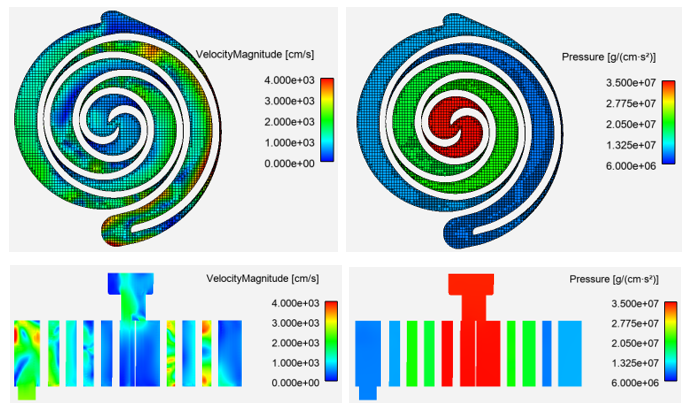
On the EnSight Part tree shown in Figure 15.3: Post-processing simulation results using EnSight, the Part VolumeCells is the one that contains the 3-D volume solutions. It can be used for creating clip-planes, iso-surfaces, particle traces, etc. Figure 15.4: Sample Forte simulation results on clip planes in EnSight shows pressure and velocity plotted on clip planes. In this example, the top two are XY clip planes (using VolumeCells as the parent) at Z = 26.5 cm, in which the mesh lines are shown as well; the bottom two are YZ clip planes at X = 0.0 cm.