This tutorial describes how to use Ansys Forte CFD to simulate the gas flow in a rotary compressor.
A non-proprietary generic geometry with a single vane is used in this tutorial as an example. The simulation methodology, conventions, and best practices also apply to other variations of this compressor. The geometry provided in this tutorial is used only for demonstrating the simulation setup using Forte and should not be used as a guidance for actual machine design.
This tutorial first explains the methodology and conventions used in a compressor simulation, and then goes through all the simulation setup steps, with emphasis on the following aspects that are unique or important to compressors:
Requirements for surface geometry preparation.
Small gap handling using gap refinement controls and the gap model.
Rotational motion setup and prescribed boundary motion for the vane.
Simulation preview for checking boundary motion and potential surface intersection.
Visualization of simulation results.
The following sections describe the prerequisites, provided files, time required, and a utility for comparing your generated project file (.ftsim) with the one provided in the tutorial download.
This tutorial will cover all the set-up steps, but we recommend that you work through the Forte Quick Start Guide first and become familiar with the workflow of the Ansys Forte user interface.
The files for this tutorial are obtained by downloading the
rotary_compressor.zip file
here .
Unzip rotary_compressor.zip to your working folder.
Files provided in this tutorial include a Forte project file that has been fully configured as well as the surface geometry input files that can be used to set up the Forte project. Specifically, the files include:
Rotary_Compressor_Tutorial.ftsim: The fully configured Forte project file.
Rotary_Compressor_Surface_Geometry.stl: Surface mesh in .stl format.
sine.csv: Prescribed sinusoidal movement of the vane starting from the retracted position for a full revolution of the geometry.
The tutorial sample compressed archive is provided as a download. You have the opportunity to select the location for the file when you download and uncompress the sample files.
Note: This tutorial is based on a fully configured sample project that contains the tutorial project settings. The description provided here covers the key points of the project set-up but is not intended to explain every parameter setting in the project. The project files have all custom and default parameters already configured; the text highlights only the significant points of the tutorial.
The installation includes the cgns_util export command, which you can use to compare the parameter settings in the project file generated at any point during your tutorial set-up against the provided .ftsim, which has the parameter settings for the final, completed tutorial. This command is described in the Forte User's Guide.
Briefly, you can double-check project settings by saving your project and then running the cgns_util to export your tutorial project, and then to export the provided final version of the tutorial. Save both versions and compare them with your favorite diff tool, such as DIFFzilla. If all the parameters are in agreement, you have set up the project successfully. If there are differences, you can go back into the tutorial set-up, re-read the tutorial instructions, and change the setting of interest.
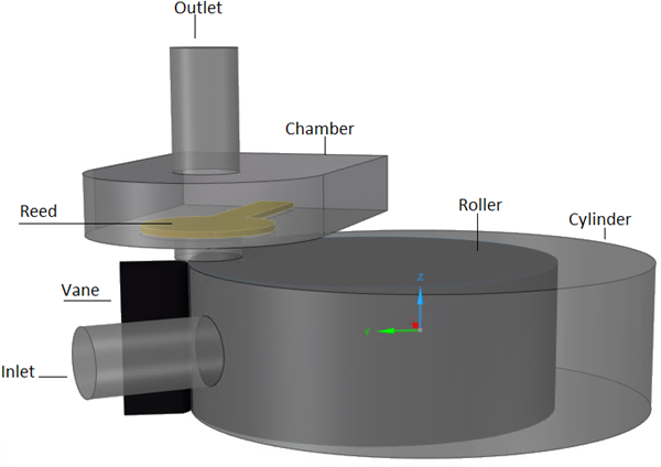
The geometry and working principle of the rotary compressor are illustrated in Figure 14.1: Configuration of the rotary compressor case. The working fluid is a 50% mix (in mass fraction) of R125 and R32 refrigerants. The cylinder and roller define the changing volume where the fluid is compressed. Each revolution lasts 0.0167 s, during which the roller compresses the fluid, the pressure builds up at the bottom of the chamber, and the reed valve eventually opens. The flow can now expand into the chamber and be released through the outlet.
Throughout the revolution, the roller is in close contact with the cylinder and the vane front, with a 10 µm gap between these surfaces. The gap between the closed reed valve and the bottom of the chamber wall is slightly larger and measures 1 µm. The vane motion is of a sinusoidal shape with the same period as the roller and the amplitude given by the eccentricity of the roller with respect to the cylinder. The movement of the reed is computed with Forte's Built-in FSI feature. The pressure difference between inlet and outlet is set at 11 bar.
The project setup workflow follows the top-down order of the workflow tree in the Ansys Forte Simulate interface. The components irrelevant to the present project will not be mentioned in this document, and you can simply skip them and use the default model options.
This tutorial uses Forte's on-the-fly automatic mesh generation (AMG) feature, which only requires the surface geometry as an input. The volume mesh does not need to be created beforehand.
Due to the nature of these compressors, where curved surfaces and tiny gaps are involved, it is extremely important that the curved surfaces are sufficiently smooth to avoid intersections during the rotation. For this reason, when exporting the surface mesh file from Ansys Discovery, we recommend choosing the Fine option for the Facet Resolution of the surface mesh file. The Angle resolution should not be much larger than 4°.
In Forte, the normal vectors of the triangulated surface mesh are required to point towards the exterior of the fluid domain. The normals of the internal solids (reed, roller and vane) should be inverted either in Discovery before exporting the surface mesh file or in Forte. The provided surface geometry file has already the normals inverted.
Now, let's proceed importing the geometry into the Forte Simulate user
interface. Go to the Geometry node and click on
Import Geometry ![]() , select the Surfaces from STL file
option, pick the file Rotary_Compressor_Surface_Geometry.stl
and choose cm as units. Accept all the default options on the
Import Options wizard window. Ensure that the Invert
Normals box is not checked, as the normals have already been properly
modified such that the surface normals of the reed, roller and vane point to the
exterior of the solids.
, select the Surfaces from STL file
option, pick the file Rotary_Compressor_Surface_Geometry.stl
and choose cm as units. Accept all the default options on the
Import Options wizard window. Ensure that the Invert
Normals box is not checked, as the normals have already been properly
modified such that the surface normals of the reed, roller and vane point to the
exterior of the solids.
We will use two different Reference Frames. The
Global Origin will be used for the roller, and it does not need
to be modified. The reed will have its own reference frame. Go to
Geometry > Reference Frames, click the
New Reference Frame ![]() icon and name it Reed Frame. The origin is
located at the base of the reed, X = 20.183349 mm, Y
= 10.079896 mm and Z = 8.05 mm. The orientation is
set to -23.545529 degrees about the Z-axis and 0
degrees around X- and Y-axis.
icon and name it Reed Frame. The origin is
located at the base of the reed, X = 20.183349 mm, Y
= 10.079896 mm and Z = 8.05 mm. The orientation is
set to -23.545529 degrees about the Z-axis and 0
degrees around X- and Y-axis.
Before moving to the mesh controls, it is appropriate to create a sub-volume to make sure the connectivity between the main domain and the discharge chamber is preserved even when the valve is in its closed position. To do so, go to Geometry > Sub-Volumes > New Sub-Volume. Name it discharge-chamber while selecting the chamber_bottom, chamber_bottom_reed, chamber_wall, outlet, outlet_port, ring_side, and ring_top surfaces to identify the sub-region. Then set the material point to be located at X = 0.35 cm, Y = 1.719 cm, and Z = 1.12 cm and click on Apply
Automatic mesh generation in Forte requires you to specify a material point that will remain inside the fluid domain for the entire simulation, a global mesh size that serves as the reference size for mesh refinement, and other refinement controls.
Set the coordinates of the Material Point to X = -0.7 cm, Y = 1.9 cm and Z = 0.0 cm, and choose a Global Mesh Size of 0.85 mm with static refinements applied as indicated in Table 14.1: Settings for mesh control refinements. The Active property is set to Always for all the mesh controls. The Ref. Frame for the Material Point should be left as default to the Global Origin. This point is located at the inlet port to ensure it will remain within the fluid domain throughout the simulation.
Three types of refinement controls are used in this tutorial: Surface
Refinement Depth ![]() , SAM (Solution Adaptive Mesh)
, SAM (Solution Adaptive Mesh) ![]() , and Gap Feature Control
, and Gap Feature Control ![]() . Detailed mesh control parameters are listed in Table 14.1: Settings for mesh control refinements. For the three Gap Feature
Controls, leave the Surface Proximity Option to the
default Determine from Surface Depth option, leave the
Surface alignment threshold to the default 45
degrees and check the box for the Enable Gap Model
option. For the gap between the reed and the ring at the bottom of the chamber wall
(reed_ring), check the Block Flow Across Gap option. Notice
that as a rule of thumb for good practices, the gap size should be on the order of
the mesh size of the surfaces where it is applied before applying the Gap
Feature Controls. For this case, the global mesh size is 0.85
mm, and the reed and the ring walls have a 1/8 refinement applied to the
surfaces where the gap is located. Then, the gap surface proximity could be set as
1.5*(1/8)*0.85 mm = 0.16 mm at the reed/ring gap to ensure the
gap size is larger than the local cell refinement. However, the Surface
Proximity Option with the Determine from Surface
Depth option selected will take care of this automatically and it is
recommended to use this option according to best practices. In gaps relating to
surfaces with FSI, it is also recommended to check Block Flow Across
Gap. See Mesh Controls for Automatic Meshing in the Ansys Forte User's Guide for
more details.
. Detailed mesh control parameters are listed in Table 14.1: Settings for mesh control refinements. For the three Gap Feature
Controls, leave the Surface Proximity Option to the
default Determine from Surface Depth option, leave the
Surface alignment threshold to the default 45
degrees and check the box for the Enable Gap Model
option. For the gap between the reed and the ring at the bottom of the chamber wall
(reed_ring), check the Block Flow Across Gap option. Notice
that as a rule of thumb for good practices, the gap size should be on the order of
the mesh size of the surfaces where it is applied before applying the Gap
Feature Controls. For this case, the global mesh size is 0.85
mm, and the reed and the ring walls have a 1/8 refinement applied to the
surfaces where the gap is located. Then, the gap surface proximity could be set as
1.5*(1/8)*0.85 mm = 0.16 mm at the reed/ring gap to ensure the
gap size is larger than the local cell refinement. However, the Surface
Proximity Option with the Determine from Surface
Depth option selected will take care of this automatically and it is
recommended to use this option according to best practices. In gaps relating to
surfaces with FSI, it is also recommended to check Block Flow Across
Gap. See Mesh Controls for Automatic Meshing in the Ansys Forte User's Guide for
more details.
Table 14.1: Settings for mesh control refinements
| Item | Refinement type | Refinement location | Refinement level | Refinement layers |
|---|---|---|---|---|
| roller_cylinder_gap |
Gap Feature Surface Proximity Option = Determine from Surface Depth; Gap Model = Enabled; Surface Alignment Threshold = 45 deg | cylinder_side, roller_side | 1/4 | |
| roller_cylinder_side | Surface | cylinder_side, roller_side | 1/4 | 1 |
| vane | Surface | vane_front, vane_slot, wall_slot | 1/4 | 1 |
| SAM_velGradient |
SAM Quantity Type = Gradient of Solution Field; Solution Variables = VelocityMagnitude; Bounds = Statistical; Sigma Threshold = 0.5 | Entire Domain | 1/2 | |
| roller_vane_gap |
Gap Feature Surface Proximity Option = Determine from Surface Depth; Gap Model = Enabled; Surface Alignment Threshold = 45 deg | roller_side, vane_front | 1/4 | |
| reed_ring |
Gap Feature Surface Proximity Option = Determine from Surface Depth; Gap Model = Enabled; Surface Alignment Threshold = 45 deg | ring_top, reed_bottom | 1/8 | |
| reed | Surface | reed_bottom, reed_side, reed_top, chamber_bottom_reed | 1/8 | 2 |
| discharge_port | Surface | discharge_port | 1/4 | 1 |
| open_boundaries | Surface | inlet, outlet | 1/4 | 1 |
| walls | Surface |
chamber_bottom, chamber_bottom_reed, chamber_wall, cylinder_bottom, cylinder_side, cylinder_top, discharge_port, inlet_port, outlet_port, roller_bottom, roller_side, roller_top, vane_front, vane_slot, wall_slot | 1/2 | 1 |
| ring | Surface | ring_side, ring_top | 1/8 | 1 |
| top_and_bottom | Surface |
cylinder_bottom, cylinder_top, roller_bottom, roller_top | 1/8 | 1 |
The Gap Feature Control is a mesh refinement control that is especially useful for handling the small gaps in compressors. This control automatically detects small gaps between the specified surface pair. When Gap Feature Control is used, the spatially resolved solution will contain a variable called GapCellFlag, which uses non-zero integer values to mark the zones identified as gap zones.
There is a 1 µm distance tolerance between the top and bottom surfaces of the roller and cylinder, as well as the vane and the vane slot walls. Forte will ignore these tiny gaps by default. However, if the end gaps are large enough and it is of interest to model the flow leakage through them, you can use the Gap Feature Control to mesh these gaps.
In Forte, a chemistry set in Chemkin format is used to define the properties
of the working fluid. The chemistry input file used in this tutorial contains
refrigerant R410A, which is composed of 50% (by mass) R125 and 50% R32 refrigerants.
Assign the chemistry with Models >
Chemistry/Materials, and use the New Import
Chemistry ![]() icon and select the file Refrigerants.cks
from the Ansys Forte data directory.
icon and select the file Refrigerants.cks
from the Ansys Forte data directory.
Forte has both ideal gas and real gas model options. To turn on the ideal gas model option, choose Real Gas as the Equation of State option on the Models > Chemistry/Materials panel.
This tutorial uses the RANS RNG k-ε turbulence model, which is the default turbulence model option. Other turbulence modeling options are available under Models > Transport > Turbulence.
Boundary conditions must be specified for each of the surfaces found in the Geometry node. To match the provided project, follow these instructions for each boundary condition:
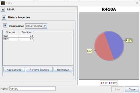
inlet: Defined as an inlet boundary ![]() . For Composition on the inlet setup panel,
select Create a new gas mixture to create a mixture called
R410A, and add species R32 and R125 with 0.5 mass fraction as
shown in Figure 14.2: Flow Composition of R410A. In general, in the chemistry
mechanism input file, cloning species with different names (such as R410A_in and
R410A_out) and assigning them to inlet and outlet boundary conditions may be used to
track the composition of reverse flow in open boundaries. However, this is not
needed for the purposes of this tutorial, and a single composition is defined for
the inlet, outlet and initial condition. Proceed to pick the
inlet surface as the selected Location,
set the Total Pressure to 9 bar, leave the
Turbulent Kinetic Energy and Length Scale
at their default values, and finally set the Total Temperature
to 20 C.
. For Composition on the inlet setup panel,
select Create a new gas mixture to create a mixture called
R410A, and add species R32 and R125 with 0.5 mass fraction as
shown in Figure 14.2: Flow Composition of R410A. In general, in the chemistry
mechanism input file, cloning species with different names (such as R410A_in and
R410A_out) and assigning them to inlet and outlet boundary conditions may be used to
track the composition of reverse flow in open boundaries. However, this is not
needed for the purposes of this tutorial, and a single composition is defined for
the inlet, outlet and initial condition. Proceed to pick the
inlet surface as the selected Location,
set the Total Pressure to 9 bar, leave the
Turbulent Kinetic Energy and Length Scale
at their default values, and finally set the Total Temperature
to 20 C.
outlet: The outlet should be defined as an inlet boundary ![]() as well to impose the reverse flow composition and temperature.
For Composition, select the R410A created
previously. Select the outlet surface for
Location. Choose the Total Pressure
option for Inlet type and set the Pressure
to 20 bar. Keep the default Turbulence
parameters. Choose Total Temperature as the
Temperature Option and set the temperature to 100
C.
as well to impose the reverse flow composition and temperature.
For Composition, select the R410A created
previously. Select the outlet surface for
Location. Choose the Total Pressure
option for Inlet type and set the Pressure
to 20 bar. Keep the default Turbulence
parameters. Choose Total Temperature as the
Temperature Option and set the temperature to 100
C.
roller: Defined as a wall boundary ![]() with wall motion. Select the
roller_bottom, roller_side and
roller_top surfaces for Location. Turn off
Heat Transfer to model the walls as adiabatic. Turn on
Wall Motion and set Motion Type as
Rotation. The rotation axis requires an
Origin and a Direction vector as the
inputs. They can be specified in an arbitrary way, but in this case the motion is
prescribed with respect to the Global Origin Reference Frame,
with coordinates X = 0.0 cm, Y = 0.0 cm,
Z = 0.0 cm, and the Z-axis (X = 0.0,
Y = 0.0, Z = 1.0) of this reference frame
for Axis Direction. Note that the rotation direction follows
the right-hand rule. Set Angular Velocity to 3,600
RPM, which corresponds to a period for a full revolution of
0.0167 s.
with wall motion. Select the
roller_bottom, roller_side and
roller_top surfaces for Location. Turn off
Heat Transfer to model the walls as adiabatic. Turn on
Wall Motion and set Motion Type as
Rotation. The rotation axis requires an
Origin and a Direction vector as the
inputs. They can be specified in an arbitrary way, but in this case the motion is
prescribed with respect to the Global Origin Reference Frame,
with coordinates X = 0.0 cm, Y = 0.0 cm,
Z = 0.0 cm, and the Z-axis (X = 0.0,
Y = 0.0, Z = 1.0) of this reference frame
for Axis Direction. Note that the rotation direction follows
the right-hand rule. Set Angular Velocity to 3,600
RPM, which corresponds to a period for a full revolution of
0.0167 s.
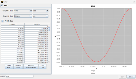
vane_front: Defined as a wall boundary ![]() with wall motion. Select the vane_front
surface for Location. Turn off Heat
Transfer to model the wall as adiabatic. Turn on Wall
Motion and set Motion Type as Offset
Table and the Timing Option as
Time. In Lift Profile, select
Create new and either load the provided
sine.csv file with the prescribed movement of the vane or
directly copy the valued as shown in Figure 14.3: Movement profile of the vane. Make sure the units are seconds
and cm and name the profile sine and save it. Make sure that
Treat Profile As Cyclic is checked. The direction should be set
to the Y-axis (X = 0.0, Y = 1.0,
Z = 0.0). Set the Movement Type to Sliding
Interface and select the surfaces vane_slot and
wall_slot. This prevents fluid cells from being generated
between these surfaces.
with wall motion. Select the vane_front
surface for Location. Turn off Heat
Transfer to model the wall as adiabatic. Turn on Wall
Motion and set Motion Type as Offset
Table and the Timing Option as
Time. In Lift Profile, select
Create new and either load the provided
sine.csv file with the prescribed movement of the vane or
directly copy the valued as shown in Figure 14.3: Movement profile of the vane. Make sure the units are seconds
and cm and name the profile sine and save it. Make sure that
Treat Profile As Cyclic is checked. The direction should be set
to the Y-axis (X = 0.0, Y = 1.0,
Z = 0.0). Set the Movement Type to Sliding
Interface and select the surfaces vane_slot and
wall_slot. This prevents fluid cells from being generated
between these surfaces.
reed: Defined as a stationary wall boundary ![]() . Select the surfaces that composes the reed,
reed_bottom, reed_top and
reed_side. For the Built-in FSI setup, the surfaces of the reed
have to be jointly defined as a separate boundary condition. Turn off Heat
Transfer to model the wall as adiabatic. Make sure that the
Roughness Height is set to 0.
. Select the surfaces that composes the reed,
reed_bottom, reed_top and
reed_side. For the Built-in FSI setup, the surfaces of the reed
have to be jointly defined as a separate boundary condition. Turn off Heat
Transfer to model the wall as adiabatic. Make sure that the
Roughness Height is set to 0.
walls: The rest of the walls can be jointly defined as a
single stationary wall boundary ![]() . Select the chamber_bottom,
chamber_bottom_reed, ring_side,
ring_top, inlet_port,
discharge_port, vane_slot,
wall_slot, cylinder_top,
cylinder_bottom, cylinder_side,
chamber_wall and outlet_port surfaces for
Location. Make sure that the Heat Transfer
is turned off and Roughness Height is set to
0.
. Select the chamber_bottom,
chamber_bottom_reed, ring_side,
ring_top, inlet_port,
discharge_port, vane_slot,
wall_slot, cylinder_top,
cylinder_bottom, cylinder_side,
chamber_wall and outlet_port surfaces for
Location. Make sure that the Heat Transfer
is turned off and Roughness Height is set to
0.
In the Initial Conditions under Default Initialization, use the same mixture as the inlet composition in Figure 14.2: Flow Composition of R410A. Set the Temperature to 20 C, the Pressure to 9 bar, the Initialization Order to 2, and leave the Turbulent Kinetic Energy and Length Scale at their default values. Now initialize the discharge chamber as a New Secondary Region From Sub-Volume, set an Initialization Order of 1, set Region Type as Other, use the same composition of R410A mentioned before, then set Temperature and Pressure as 100 C and 20 bar respectively. Leave everything else as default.
Simulation Limits: Choose the Time Based option to specify the Simulation End Point and set Max. Simulation Time to 0.0167 s. This duration covers one complete revolution of the roller.
Time Step: Forte uses adaptive time step controls to adjust the actual time step size for each transient flow integration step. The user-specified max time step will be used if the time step is not subject to other constraints listed under Advanced Time Step Control Options. For rotating machinery simulation, the rule of thumb for choosing the Max. Simulation Time Step is to have at least 10 time steps per degree of rotation of the fastest rotating motion in the system. Using this guideline, the Max Time Step can be estimated as 60/(RPM*360*10) = 1/(RPM*60) s, which gives roughly 4.6E-6 s for RPM = 3,600. In this tutorial, the Max Time Step is set to 2E-6 s, which is a conservative choice based on this calculation. For the Advanced Time Step Control Options, typically it is acceptable to relax the Fluid Acceleration Factor and Rate of Strain Factor to achieve larger time steps without affecting the accuracy and stability very much. In this calculation, these two factors are set to 1.0 and 1.2, respectively. Both are two times their default values. It is risky to change the other control factors because relaxing them may cause the solution to become unstable.
Chemistry Solver: Set the Activate Chemistry option to Always Off because this simulation does not involve chemical kinetics.
Built-in FSI: The movement of Reed is going to be modeled by the built-in FSI feature in Forte. Check Built-in FSI in the Simulation Controls node and add a New Beam Bending. Select the reed for Location. The Youngs's Modulus is set to 28 GPa. Turn on Enable Inertial and Damping Effects and set the Mass of Body to 0.239 g and Damping Coefficient to 10 dyne-cm-sec/degree. Select the Load Type as Partial Distributed Load with L1/L set to 0.4, and check the Restrict Positive Displacement box with 0.01 mm Displacement Threshold, 2.75 mm Maximum Displacement, and 0.05 Max. Travel Per Step. For Fixed End Position, select the Reed Frame as the Ref. Frame and set the location to X = 0.0 cm, Y = 0.0 cm and Z = 0.0 cm. The Neutral Axis is also defined with respect to the Reed Frame, and in the negative X-axis (X = -1.0 cm, Y = 0.0 cm, Z = 0.0 cm). The Beam Axis, which is the axis of rotation of the beam, is also defined with respect to the Reed Frame, and in the positive Y-axis (X = 0.0 cm, Y = 1.0 cm and Z = 0.0 cm).
Spatially Resolved: Use Time as the Output Timing Control option. Set Interval Based Output Control to output every 0.002778 s, which corresponds to a sixth of a revolution. A user defined list of times of interest to save the spatially resolved solution can be created turning on the User Defined Output Controls and creating a time list. For the Spatially Resolved Species list, select R32 and R125. For the Solution Variables list, select variables of interest. The minimum variable set should include Pressure, Temperature, VelocityX, VelocityY, VelocityZ, and VelocityMagnitude.
Spatially Averaged And Spray: Choose the Time option and set the output interval to 5.0E-5 s. Select R32 and R125 in the Spatially Averaged Species list. Check the Enable Time Averaging Output box at the bottom of the editor panel and pick the Time Averaging Option of your choice. It is good practice to discard the first revolution and start averaging after that. In this tutorial we only simulate 1 revolution, so we keep the default option of Use All Time Points.
Restart Data: Make sure Write Restart File at Last Simulation Step is checked ON. This option allows a restart file to be saved at the end of the current simulation. Such a restart file is useful if you decide to extend the simulation duration to do parameter studies because it provides a much better guess for initial condition than a uniform one. This practice may help save CPU time spent in simulating the initial transient process. Turn on Interval Based Restart and set the Output Timing Control to Time. Then set the Time Interval Between Restart Dumps to 0.008333 s, so that it will save a restart file every half revolution. This type of restart file can help provide a recovery point if a long-running job was unexpectedly interrupted.
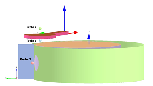
Monitor Probes: On the Monitor Probes setup panel, for the
Inquiry Frequency, choose Time as the
Frequency Option and set the interval to 5.0E-5
s. Click the New Probe icon ![]() to add three new monitor probes named Probe
1, Probe 2 and Probe 3. The
three of them have the following settings:
to add three new monitor probes named Probe
1, Probe 2 and Probe 3. The
three of them have the following settings:
Monitor Type: Geometric.
Geometric Shape: Spherical.
Solution Variables selected: Pressure and Temperature
Active: Always.
Location: Constant.
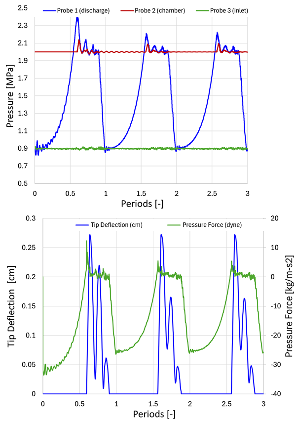
The locations with respect to the Global Origin are (X = 0.35 cm, Y = 1.719 cm, Z = 0.72 cm), (X = 0.35 cm, Y = 1.719 cm, Z = 1.12 cm), and (X = -0.7 cm, Y = 1.9 cm, Z = 0.0 cm), for the probes 1 to 3 respectively. Set the Radius to 0.05 cm. The locations of the probes can be seen in Figure 14.4: Probe locations.
Additional Output: Forte offers the possibility to have an additional or an alternative set of output format, namely EnSight DVS (Dynamic Visualization Store), which allows to save spatially resolved solutions in an efficient manner, reducing the loading time and the stepping through transient solution points in Ansys EnSight. Also, better performance during solution writing especially when running a job on a cluster with many processors. To use the EnSight DVS format, start by clicking the EnSight icon on the Additional Output editor panel. Then check the Enabled box under EnSight DVS Settings.
For the EnSight DVS settings, use Time as the Output Timing Control option. Set Interval Based Output Control to output every 0.002778 s, which corresponds to a sixth of a revolution. A user defined list of times of interest to save the spatially resolved solution can be created by turning on the User Defined Output Controls and creating a time list (which is not used in this tutorial). For the Spatially Resolved Species list, select R32 and R125. For the Solution Variables list, select variables of interest. The minimum variable set should include Pressure, Temperature, VelocityX, VelocityY, VelocityZ, and VelocityMagnitude. For the purpose of this tutorial, the default Solution Variables and Spatially Averaged Variables are sufficient. Make sure the Forte's Spatially Resolved option is not checked in the Output Controls node because the DVS option is used instead.
Note: If you fail to select the Enabled box, no EnSight DVS output will be generated, even if the rest of the panel is properly set. DVS output can be enabled independently from Forte's spatially resolved output. Therefore, it often makes sense to disable Forte's spatially resolved output when using DVS.
The DVS results will be contained in a subfolder of the run directory, named according to the user-supplied name of the DVS output added to the Workflow tree. To load the results in EnSight, within an EnSight session, choose File > Open and select the .dvs file from this directory or use the EnSight launcher shortcut on Forte's Run panel, which will search for and provide a list of available .dvs files in the analysis directory that can be preselected and passed to the newly launched EnSight instance.
To detect potential problems due to surface intersection or mesh generation before the simulation is started, navigate to the Preview Simulation node. On the Mesh Generation panel, set the Time Option to Time for investigating a specific Time or to Time Range for a more extensive investigation, then select Check for Surface Intersections and/or Include Volume Mesh (highly recommended for a case with moving parts), and finally launch the preview by clicking the Generate Mesh icon. It is a good idea to create a mesh preview with multiple steps spanning over an entire revolution to check the mesh quality across the full rotation. In the Mesh Generation editor panel, you can also select how many cores to use when performing this mesh check by changing the MPI Arguments under the Run Options. The Preview of the movement in EnSight is shown in Figure 14.5: Preview simulation output.
The run settings depend on the system and environment for your simulations. Change the number of cores to use for this simulation according to the resources available to you by navigating to Run Settings > Run Options, and under Job Script Options, setting the number of cores for Default MPI Arguments. No other changes are needed, and you can continue launching the simulation.
This final section of the tutorial is dedicated to the collection of the results. In Figure 14.6: Mesh evolution and spatially resolved velocity and pressure, you can see at the top left side the mesh evolution on a vertical and horizontal cut plane. At the top right side, the pressure is reported on the same clip planes. The two zoomed views of the surroundings of the reed at the bottom show the velocity magnitude streamlines (bottom left) and the pressure contour (bottom right). When the pressure below the reed meets a certain threshold, the reed opens, and the flow discharge occurs. Notice the flow blockage at the bottom of the reed valve holds the pressure difference between the two main regions at different pressure
The spatially averaged solutions are reported in CSV format in the run folder (Nominal). Ansys Forte Monitor is a convenient tool for displaying these averaged solutions, or any other program of choice can be used to plot the data in CSV format. In Figure 14.7: Spatially averaged results, spatially averaged results are plotted. The movement of the reed is depicted along with the resulting force at the reed. The pressure on the probes is also shown.