This tutorial targets the Sandia's optical hydrogen engine (SOpHy) in its "low tumble" configuration with H2 direct injection. Original geometry and measurements data can be downloaded directly from the Engine Combustion Network here Hydrogen Engine – Engine Combustion Network (sandia.gov).
The following sections describe the provided files, time required, prerequisites, and a utility for comparing your generated project file (.ftsim) with the one provided in the tutorial download.
This tutorial will cover all the set-up steps, but we recommend that you work through the Forte Quick Start Guide first and become familiar with the workflow of the Ansys Forte user interface.
The files for this tutorial are obtained by downloading the
h2_engine.zip file
here .
Unzip h2_engine.zip to your working folder.
Files provided in this tutorial include a Forte project file that has been fully configured as well as the surface geometry input files that can be used to set up the Forte project. Specifically, the files include:
LT_wInj_Tutorial.ftsim: the fully configured Forte project file.
LT_wInj_Tutorial.stl: the surface geometry input file.
Pressure_inlet.csv: the inlet pressure profile.
Pressure_outlet.csv: the inlet pressure profile.
INprofile_0.5.csv: the intake valves lift profile.
EXprofile_0.5.csv: the exhaust valves lift profile.
H2inlet_MassFlowRate.csv: the injected hydrogen mass flow rate profile.
The tutorial sample file is provided as a download. You have the opportunity to select the location for the file when you download and uncompress the sample files.
Note: This tutorial is based on a fully configured sample project that contains the tutorial project settings. The description provided here covers the key points of the project setup but is not intended to explain every parameter setting in the project. The project files have all custom and default parameters already configured, the text highlights only the significant points of the tutorial.
The installation includes the cgns_util export command, which you can use to compare the parameter settings in the project file generated at any point during your tutorial set-up against the provided .ftsim, which has the parameter settings for the final, completed tutorial. This command is described in the Forte User's Guide.
Briefly, you can double-check project settings by saving your project and then running the cgns_util to export your tutorial project, and then to export the provided final version of the tutorial. Save both versions and compare them with your favorite diff tool, such as DIFFzilla. If all the parameters are in agreement, you have set up the project successfully. If there are differences, you can go back into the tutorial set-up, re-read the tutorial instructions, and change the setting of interest.
Hydrogen combustion in engines exhibits quite different characteristics than hydrocarbon fuels, and the optimization of potential fuel blends and engine design will involve engine modeling. In this tutorial, we have explored best practices for CFD modeling of direct-injection hydrogen IC engines. As a first step we present a non-firing case with hydrogen injection, focusing on flow and mixing effects. For this, we have used Sandia ECN data for validation.
The project setup workflow follows the top-down order of the workflow tree in the Ansys Forte Simulate interface. The components irrelevant to the present project will not be mentioned in this document, and you can simply skip them and use the default model options.
One of the main advantages of using Forte in your simulation is that you
don’t need to create the volume mesh beforehand, since it will be
automatically generated on-the-fly. Instead, you only need to create a surface mesh
and import it in Forte. For this tutorial we provide the surface mesh in the
.stl format exported from the CAD geometry in Ansys Discovery, that
you need to import in the Forte UI. Go to the Geometry node
and click on Import Geometry ![]() , select the Surface from one or more STL
files option, pick your file or the
LT_wInj_Tutorial.stl and choose cm as
units. Note that once you have imported the geometry, there are a number of actions
that you can perform to modify the geometry elements, such as scale, rename,
transform, invert normals, or delete. It is important at this stage that the
imported engine geometry has the piston at its top dead center independently from
the initial crank angle of the simulation. This facilitates the stretching of the
mesh and allows the piston to slide all the way down to the bottom dead
center.
, select the Surface from one or more STL
files option, pick your file or the
LT_wInj_Tutorial.stl and choose cm as
units. Note that once you have imported the geometry, there are a number of actions
that you can perform to modify the geometry elements, such as scale, rename,
transform, invert normals, or delete. It is important at this stage that the
imported engine geometry has the piston at its top dead center independently from
the initial crank angle of the simulation. This facilitates the stretching of the
mesh and allows the piston to slide all the way down to the bottom dead
center.
Note: If you want to create the surface mesh yourself, we recommend using the option Fine and 4° for the Facet and AngleResolution, respectively, when exporting the .tgf file from Ansys Discovery. The reason being that the gear and casing geometries have curved surfaces in 3-D with tiny gaps in between therefore the curved surfaces are required to be sufficiently smooth to avoid unwanted surface intersections during their motion.
Create now 3 new Reference Frames for an easier setup later on in the workflow tree. See Table 8.1: Reference Frames in cartesian coordinates for further details on their cartesian coordinates.
Table 8.1: Reference Frames in cartesian coordinates
| Reference Frame | X [cm] | Y [cm] | Z [cm] | X-rotation [deg] | Y-rotation [deg] | Z-rotation [deg] |
|---|---|---|---|---|---|---|
|
EXvalves |
-3.162 |
4.077 |
1.937 |
0 |
0 |
22.05 |
|
INvalves |
3.307 |
5.25 |
1.95 |
0 |
0 |
-20 |
|
Injector |
-0.51472 |
1.495974 |
0.000321 |
0 |
0 |
-130 |
Once you have imported the geometry, go to the Sub-volume node, create a New Sub-Volume and label it chamber. The selected surfaces bounding the new sub-volume are crevice_bottom, crevice_side, head, liner and piston. Chose the sub-volume material point to be at X = 0 cm, Y = 0.5 cm, Z = 0 cm in cartesian coordinates, and select the Multiple passes as the Capping Method.
It is always useful to create a Clip Plane to double check that the material point lays within the watertight geometry. Create one centered at the origin with -z as the plane normal.
To allow the mesh generation on-the-fly, you are required to setup the material point inside the fluid domain. For geometries with moving boundaries, like the one in this tutorial, you also want to make sure the material point will remain within the domain throughout the simulation. For this reason, we placed the material point between the injector and the piston at its top dead center.
The coordinates of the Material Point are: X = 0 cm, Y = 0.5 cm, Z = 0 cm, and we chose a Global Mesh Size of 2 mm with static refinements applied as indicated in Table 8.2: Mesh refinements settings.
Among the Mesh controls there is an additional dynamic refinement type, the
Gap Feature Control ![]() , applied to the crevice_side and
liner. This type of refinement is of key importance when small
gaps are present. In its editor panel setting, you are asked to indicate a
Surface Proximity that will identify the gap between the pair
of surfaces selected in the Location box. For this tutorial we
set the Surface Proximity to be 12 mm and
the refinement level for those cells within the gap to ½
of the global mesh size.
, applied to the crevice_side and
liner. This type of refinement is of key importance when small
gaps are present. In its editor panel setting, you are asked to indicate a
Surface Proximity that will identify the gap between the pair
of surfaces selected in the Location box. For this tutorial we
set the Surface Proximity to be 12 mm and
the refinement level for those cells within the gap to ½
of the global mesh size.
Starting from 2024 R1, it is possible to modify the angular deviation between faces forming a gap. A value of zero indicates the faces bounding a gap must be parallel, a higher value is more permissive and will detect more gap cells. For this tutorial we kept the default value. In the same editor panel check the Enable Gap Model box to compensate for the under-resolution in the gap zones. In other words, setting the refinement level to ½ of the global mesh size, indicated that the fluid cells sizes within the gap are of 1 mm which means that some of the gaps only contain a fraction of a Cartesian cell cut by the physical boundary. Therefore, by enabling the Gap Model a momentum sink term is applied, which accounts for the underpredicted wall shear stress and over-predicted mass flow rate on the coarse grid. The Gap Model takes both the gap size and the local fluid cell size as inputs, and therefore the flow solution is not expected to be very sensitive to the gap refinement level.
The last parameter to set in the Gap Feature Control editor panel is the Gap Size Scale Factor. It can be used to enlarge or shrink the gap sizes measured on the geometry. The scaled gap size is then used as the input for the gap model in each local CFD cell in the gap zone. If the gap size in the geometry accurately reflects the size in the actual gap, the best practice is to use the default value of 1.0. In this tutorial, we use the default value.
Table 8.2: Mesh refinements settings
| Refinement | Type | Location | Level | Layers | Active |
|---|---|---|---|---|---|
|
Walls |
Surface |
crevice_boom crevice_side exhaust exvalve1_skirt exvalve1_stem exvalve2_skirt exvalve2_stem head intake1 intake2 invalve1_skirt invalve1_stem invalve2_skirt invalve2_stem liner piston |
1/2 |
1 |
Always |
|
OpenBoundaries |
Surface |
inlets outlet |
1/4 |
2 |
Always |
|
Valves_Skirt |
Surface |
exvalve1_skirt exvalve2_skirt invalve1_skirt invalve2_skirt |
1/4 |
2 |
Always |
|
SAM-Velocity |
SAM Quantity Type = Gradient of Solution Field; Solution Variables = VelocityMagnitude; Bounds = Statistical; Sigma Threshold = 0.5 |
Entire Domain |
1/4 |
|
Always |
|
SAM-h2 |
SAM Quantity Type = Gradient of Species Solution Field; Species = h2; Bounds = Statistical; Sigma Threshold = 0.5 |
Sub-volume: chamber |
1/4 |
|
During Crank Angle Interval Crank Angle Option = Cyclic [-140°, 30°] |
|
Compression |
Secondary Volume |
Sub-volume: chamber |
1/2 |
|
During Crank Angle Interval Crank Angle Option = Cyclic [-140°, 50°] |
|
h2jet |
Line |
Point 1 Ref. Frame = Injector Cartesian Coordinates: X = 0 cm, Y = 0 cm, Z = 0 cm Point 2 Ref. Frame = Injector Cartesian Coordinates: X = 0 cm, Y = 6.5 cm, Z = 0 cm Radius = 0.75 cm |
1/8 |
|
During Crank Angle Interval Crank Angle Option = Cyclic [-138°, 115°] |
|
Crevice_2_Gap-feature | Gap Feature Surface Proximity = 12 mm Surface alignment threshold = 45 degrees Enable Gap Model = ON Gap Size Scale Factor = 1 |
crevice_side liner |
1/2 |
|
Always |
|
Injector |
Line |
Point 1 Ref. Frame = Injector Cartesian Coordinates: X = 0 cm, Y = 0 cm, Z = 0 cm Point 2 Ref. Frame = Injector Cartesian Coordinates: X = 0 cm, Y = 6.5 cm, Z = 0 cm Radius = 0.75 cm |
1/16 |
|
During Crank Angle Interval Crank Angle Option = Cyclic [-138°, 118°] |
|
h2jet-always |
Line |
Point 1 Ref. Frame = Injector Cartesian Coordinates: X = 0 cm, Y = 0 cm, Z = 0 cm Point 2 Ref. Frame = Injector Cartesian Coordinates: X = 0 cm, Y = 6.5 cm, Z = 0 cm Radius = 0.75 cm |
1/4 |
|
Always |
|
IVO |
Surface |
invalve1_skirt invalve1_stem invalve2_skirt invalve2_stem |
1/16 |
1 |
During Crank Angle Interval Crank Angle Option = Cyclic [-370°, -369°] |
|
IVC |
Surface |
invalve1_skirt invalve1_stem invalve2_skirt invalve2_stem |
1/16 |
1 |
During Crank Angle Interval Crank Angle Option = Cyclic [-145°, -144°] |
|
EVO |
Surface |
exvalve1_skirt exvalve1_stem exvalve2_skirt exvalve2_stem |
1/16 |
1 |
During Crank Angle Interval Crank Angle Option = Cyclic [134°, 135°] |
|
EVC |
Surface |
exvalve1_skirt exvalve1_stem exvalve2_skirt exvalve2_stem |
1/16 |
1 |
During Crank Angle Interval Crank Angle Option = Cyclic [359°, 360°] |
|
SAM-h2_2 |
SAM Quantity Type = Gradient of Species Solution Field; Species = h2; Bounds = Absolute; Lower Bound = 0.1; Upper Bound = 100 |
Sub-volume: chamber |
1/4 |
|
During Crank Angle Interval Crank Angle Option = Cyclic [-140°, 30°] |
|
Crevice_always |
Surface |
crevice_side |
1/2 |
1 |
Always |
|
Valves-Stem |
Surface |
exvalve1_stem exvalve2_stem invalve1_stem invalve2_stem |
1/2 |
2 |
Always |
A reduced version of the Ansys MFL hydrogen mechanism has been used for this case. The hydrogen mechanism Hydrogen_MFL2021.cks can be found in the MFL Skeletal mechanism folder. MFL mechanism folders can be found in InstallDirectory\reaction\data\ModelFuelLibrary (where InstallDirectory on Windows is typically C:\Program Files\ANSYS Inc\version). Starting from that mechanism, for this non-reacting case all species and their associated reactions were removed except for nitrogen (n2) and hydrogen (h2).
This tutorial uses the RANS RNG k-epsilon turbulence model, which is the default turbulence model option. Other turbulence modeling options are available under Models > Transport > Turbulence.
Boundary conditions must be specified for each of the surfaces found in the Geometry node. To match the provided project, follow these instructions for each boundary condition:
Piston: Defined as a wall boundary
 . Select the crevice_bottom,
crevice_side, and piston surfaces
for Location. Keep the Law of the
Wall as Wall Slip Condition, with the
default roughness parameters. Enable the heat transfer option and set the
Wall Temperature at 353.15 K. Then
choose the Han-Raitz-Model and enable the
Pressure and Roughness effects.
The Motion type needs to be set to Slider Crank with a
Stroke of 85 mm, a
Connecting Rod Length of 166.67 mm
and a Piston Offset of 1.57
mm, moving along the y direction.
. Select the crevice_bottom,
crevice_side, and piston surfaces
for Location. Keep the Law of the
Wall as Wall Slip Condition, with the
default roughness parameters. Enable the heat transfer option and set the
Wall Temperature at 353.15 K. Then
choose the Han-Raitz-Model and enable the
Pressure and Roughness effects.
The Motion type needs to be set to Slider Crank with a
Stroke of 85 mm, a
Connecting Rod Length of 166.67 mm
and a Piston Offset of 1.57
mm, moving along the y direction. Inlet: Defined as an inlet boundary
 . Set the Composition to be pure
N2 and select the inlets surface
for Location. Select a Total Pressure, Time
Varying option and load the pressure profile provided
Pressure_inlet.csv, and enable the Repeat
Profile Each Cycle option. Set the Total
Temperature to 36°C and leave all the
other parameters as default.
. Set the Composition to be pure
N2 and select the inlets surface
for Location. Select a Total Pressure, Time
Varying option and load the pressure profile provided
Pressure_inlet.csv, and enable the Repeat
Profile Each Cycle option. Set the Total
Temperature to 36°C and leave all the
other parameters as default.h2inlet: Defined as an inlet boundary
. Set the Composition to be pure
H2 and select the h2inlet surface
for Location. Select a Mass Flow Rate, Time
Varying option and load the mass flow rate profile provided
H2inlet_MassFlowRate.csv, and enable the
Repeat Profile Each Cycle option. Set the
Total Pressure to 100 bar and the
Total Temperature to 309.15 K and
leave all the other parameters as default.InValve2: Defined as a wall boundary
. Select the invalve2_skirt and
invalve2_stem surfaces for
Location. Keep the Law of the Wall
as Wall Slip Condition, with the default roughness
parameters. Enable the heat transfer option and set the Wall
Temperature at 353.15 K. Then choose the
Han-Raitz-Model and enable the
Pressure and Roughness effects.
Use the Offset Table option as a Motion
Type, and load the provided lift profile
INprofile_0.5.csv marking -y as
the direction of motion in the INvalves reference
frame. Pick Valve in the Movement
Type and select intake2 and
invalve2_skirt. Make sure that the Valve
Motion Activation Threshold is 0.5 mm and
the Approximated Cells in Gap are
2.InValve1: Defined as a wall boundary
. Select the invalve1_skirt and
invalve1_stem surfaces for
Location. Keep the Law of the Wall
as Wall Slip Condition, with the default roughness
parameters. Enable the heat transfer option and set the Wall
Temperature at 353.15 K. Then choose the
Han-Raitz-Model and enable the
Pressure and Roughness effects.
Use the Offset Table option as a Motion
Type, and load the provided lift profile
INprofile_0.5.csv marking -y as
the direction of motion in the INvalves reference
frame. Pick Valve in the Movement
Type and select intake1 and
invalve1_skirt. Make sure that the Valve
Motion Activation Threshold is 0.5 mm and
the Approximated Cells in Gap are
2.ExValve2: Defined as a wall boundary
. Select the exvalve2_skirt and
exvalve2_stem surfaces for
Location. Keep the Law of the Wall
as Wall Slip Condition, with the default roughness
parameters. Enable the heat transfer option and set the Wall
Temperature at 353.15 K. Then choose the
Han-Raitz-Model and enable the
Pressure and Roughness effects.
Use the Offset Table option as a Motion
Type, and load the provided lift profile
EXprofile_0.5.csv marking -y as
the direction of motion in the EXvalves reference
frame. Pick Valve in the Movement
Type and select exhaust and
exvalve2_skirt. Make sure that the Valve
Motion Activation Threshold is 0.5 mm and
the Approximated Cells in Gap are
2.ExValve1: Defined as a wall boundary
. Select the exvalve1_skirt and
exvalve1_stem surfaces for
Location. Keep the Law of the Wall
as Wall Slip Condition, with the default roughness
parameters. Enable the heat transfer option and set the Wall
Temperature at 353.15 K. Then choose the
Han-Raitz-Model and enable the
Pressure and Roughness effects.
Use the Offset Table option as a Motion
Type, and load the provided lift profile
EXprofile_0.5.csv marking -y as
the direction of motion in the EXvalves reference
frame. Pick Valve in the Movement
Type and select exhaust and
exvalve2_skirt. Make sure that the Valve
Motion Activation Threshold is 0.5 mm and
the Approximated Cells in Gap are
2.Head: Defined as a wall boundary
. Select the head and
injector surfaces for Location.
Keep the Law of the Wall as Wall Slip
Condition, with the default roughness parameters. Enable the heat
transfer option and set the Wall Temperature at
353.15 K. Then choose the
Han-Raitz-Model and enable the
Pressure and Roughness
effects.Intake_Port: Defined as a wall boundary
. Select the intake1 and
intake2 surfaces for Location.
Keep the Law of the Wall as Wall Slip
Condition, with the default roughness parameters. Enable the heat
transfer option and set the Wall Temperature at
309.15 K. Then choose the
Han-Raitz-Model and enable the
Pressure and Roughness effects.
Exhaust_Port: Defined as a wall boundary
. Select the exhaust surface for
Location. Keep the Law of the Wall
as Wall Slip Condition, with the default roughness
parameters. Enable the heat transfer option and set the Wall
Temperature at 353.15 K. Then choose the
Han-Raitz-Model and enable the
Pressure and Roughness effects.
Outlet: Defined as an outlet boundary
 . Select the outlet surface for
Location. Set the Total Pressure
to Time Varying, and load the
Pressure_outlet.csv provided profile, with the
Repeat Profile Each Cycle option. Then, let the
Turbulent Kinetic Energy and Length
Scale with their default values.
. Select the outlet surface for
Location. Set the Total Pressure
to Time Varying, and load the
Pressure_outlet.csv provided profile, with the
Repeat Profile Each Cycle option. Then, let the
Turbulent Kinetic Energy and Length
Scale with their default values.Liner: Defined as a wall boundary
. Select the liner surface for
Location. Keep the Law of the Wall
as Wall Slip Condition, with the default roughness
parameters. Enable the heat transfer option and set the Wall
Temperature at 353.15 K. Then choose the
Han-Raitz-Model and enable the
Pressure and Roughness
effects.
In the Initial Composition under Default Initialization is created with the IVC calculator utility. It imposes a mass fraction of N2 = 0.99936 and H2 = 6.39e-4. The Temperature is set to 309.15 K, the Pressure to 1 atm, the Turbulent Kinetic Energy and Length Scale to their default values. Set the initialization order to 3.
In addition to the Default initialization, there are other 3 Secondary Regions Initializations of type Other, identified by a material point. Those are reported in Table 8.3: Secondary Regions Initializations
Table 8.3: Secondary Regions Initializations
| Name | Location | Initialization Order | Composition mass fraction | Temperature | Pressure |
|---|---|---|---|---|---|
|
Exhaust |
Ref. Frame: EXvalves Cartesian Coordinates: X = 3 cm, Y = 0 cm, Z = 0 cm |
4 |
N2 = 0.993 H2 = 0.007 |
353.15 K |
0.96 bar |
|
Intake |
Ref. Frame: INvalves Cartesian Coordinates: X = 2 cm, Y = 1 cm, Z = 0 cm |
1 |
N2 = 1 |
353.15 K |
1 bar |
|
Intake2 |
Ref. Frame: INvalves Cartesian Coordinates: X = 2 cm, Y = 1 cm, Z = -4 cm |
2 |
N2 = 1 |
353.15 K |
1 bar |
Let the simulation to be Crank Angle Based and set it to run from -360 to 360 crank angle degrees. The RPM is 1500, and the Cycle Type is 4-Stroke. Everything else is as default.
In the Time Step editor panel, have the Initial Simulation Time Step to be 5e-7 sec, and the Max. Simulation Time Step to be 5e-6 sec.
In the Chemistry Solver editor panel, turn off chemistry by setting Activate Chemistry to Always Off.
Output controls determine what data are stored for viewing during the simulation and for creating plots, graphs and animations in Ansys EnSight.
Spatially Averaged and Spray: Opt for Crank Angle in the Spatially Averaged Output Control and set the interval to 0.5 degrees, then choose the species of interest if any.
Restart Data: It is good practice to enable the restart data writing at the end of a simulation in case you want continue it later. You could also choose to have restart files written at a certain frequency or at specified times depending on your needs.
Additional Output: Starting with Ansys Forte 2022 R1, alongside the standard spatially resolved outputs (.ftres format), Forte offers the possibility to have an additional or an alternative set of output format, namely EnSight DVS (Dynamic Visualization Store). The DVS format helps reduce the loading time and the stepping through transient solution points in Ansys EnSight, thanks to the smaller size of the files generated. Better performance is also expected during the solution writing, especially when running a job on a cluster with many processors. To utilize the EnSight DVS format, start by clicking the EnSight icon on the Additional Output editor panel. Then check the Enabled box under EnSight DVS Settings. The output settings follow the same structure as Forte's native spatially resolved outputs. In other words, select your Interval Based Output Control frequency and pick your Solution Variables of interest. Only those in this list will be found in EnSight, so it is always suggested to have amongst this at least Pressure and Velocity Magnitude. If you scroll down in the same EnSight DVS editor panel you can also add the Spatially Averaged Datasets in the same additional output files set.
Note: If you fail to select the Enabled box, no EnSight DVS output will be generated, even if the rest of the panel is properly set. DVS output can be enabled independently from Forte's spatially resolved output. Therefore it often makes sense to disable Forte's spatially resolved output when using DVS.
The DVS results will be contained in a subfolder of the run directory, named according to the user-supplied name of the DVS output added to the Workflow tree. To load the results in EnSight, within an EnSight session, choose File > Open and select the .dvs file from this directory or use the EnSight launcher shortcut on Forte's Run panel, which will search for and provide a list of available .dvs files in the analysis directory that can be preselected and passed to the newly launched EnSight instance.
To detect potential problems due to surface intersection or mesh generation before the
simulation is started, navigate to the Preview Simulation node. On
the Mesh Generation panel, set the Time Option
to Crank Angle for investigating a specific angle or to
Angle Range for a more extensive investigation, then select
Check for Surface Intersections and/or Include Volume
Mesh (highly recommended for a case with moving parts), and finally launch
the preview by clicking the Generate Mesh ![]() icon. In the Mesh Generation editor panel, you can also select how
many cores to use when performing this mesh check by changing the MPI
Arguments under the Run Options.
icon. In the Mesh Generation editor panel, you can also select how
many cores to use when performing this mesh check by changing the MPI
Arguments under the Run Options.
The run settings depend on the system and environment for your simulations. Change the number of cores to use for this simulation according to the resources available to you by navigating to Run Settings > Run Options, and under Job Script Options, setting the number of cores for Default MPI Arguments. No other changes are needed, and you can continue launching the simulation.
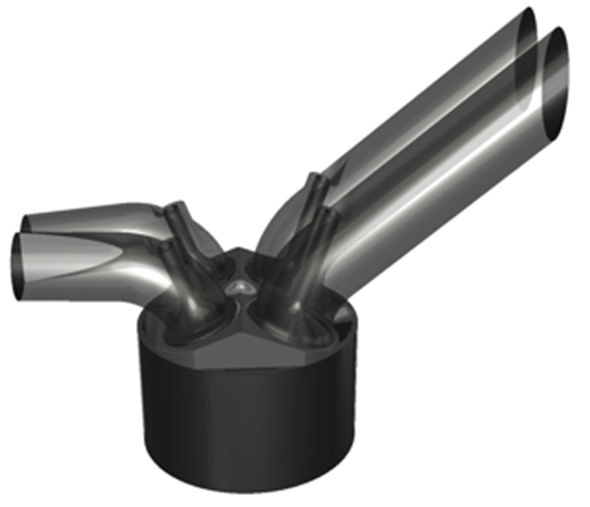
The final section of this tutorial is a collection of the results. In Figure 8.2: H2 mole fraction, temperature, and mesh evolution during compression on a Z-cut plane, you can see on the left side of the view, the evolution of H2-mole fraction on a cut plane in the middle of the z-direction. The ports are made transparent to allow a visualization of the inside and at the same time maintain the 3-dimensionality of the problem. At the top left of the animated gif notice how the mesh generated on-the-fly keeps adapting to capture both the H2 and velocity gradient. The right part of the GIF shows the temperature distribution at the same clip plane.
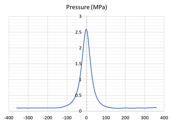
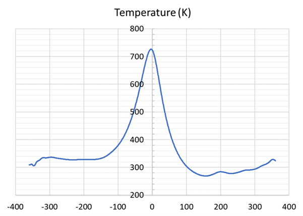
The spatially averaged in-cylinder pressure and temperature are reported in Figure 8.3: Spatially-averaged in-cylinder pressure vs. crank angle and in Figure 8.4: Spatially-averaged in-cylinder temperature vs. crank angle.