This tutorial presents the soot particle tracking capability in Ansys Forte, applying the method of moments to a diesel engine case. With the soot particle tracking feature, several spatially resolved values of soot can be simulated, including particle number density, volume fraction and average diameter. The tutorial explains the setup for using the particle tracking capability, and presents visualizations of soot predictions.
We recommend starting with the Ansys Forte Quick Start Guide, which explains the workflow of the Ansys Forte user interface, before doing this tutorial.
The files for this tutorial are obtained by downloading the
soot_particle_tracking.zip file
here
.
Unzip soot_particle_tracking.zip to your working folder.
Soot-particle-tracking__tutorial.ftsim: A project file of the completed tutorial, for verification or comparison of your progress in the tutorial set-up. The project file includes all the relevant geometry, chemistry set and spray profile details.
The tutorial sample file is provided as a download. You have the opportunity to select the location for the file when you download and uncompress the sample files.
Note: This tutorial is based on a fully configured sample project that contains the tutorial project settings. The description provided here covers the key points of the project set-up but is not intended to explain every parameter setting in the project. The .ftsim file has all custom and default parameters already configured; the text highlights only the significant points of the tutorial.
Forte may be launched in a command line mode to perform certain tasks such as preparing a run for execution, importing project settings from a text file, or various other tasks described in the Forte User's Guide. One of these tools allows exporting a textual representation of the project data to a text file.
Example
forte.sh CLI -project <project_name>.ftsim -export tutorial_settings.txt
Briefly, you can double-check project settings by saving your project and then running the command-line utility to export the settings in your tutorial project (<project_name>.ftsim), and then use the command a second time to export the settings in the provided final version of the tutorial. Compare them with your favorite diff tool, such as DIFFzilla. If all the parameters are in agreement, you have set up the project successfully. If there are differences, you can go back into the tutorial set-up, re-read the tutorial instructions, and change the setting of interest.
The Soot-particle-tracking__tutorial.ftsim project file has been preconfigured with all the information that will be discussed in this section. You do not need to input any values but can just follow along, reading the instructions and viewing the settings in the loaded .ftsim. This chapter nevertheless explains step-by-step the process of setting up the project, as an illustration of the features in the user interface.
Open the project file, Soot-particle-tracking__tutorial.ftsim, from the location where you stored the downloaded tutorial files.
A simple engine configuration is used in this tutorial for demonstration purposes. The details of the configuration and simulation settings are presented in Table 6.1: Details of the diesel engine geometry used in this tutorial.
Table 6.1: Details of the diesel engine geometry used in this tutorial
|
Compression ratio |
15 |
|---|---|
|
Displacement volume (cm3) |
508.7 |
|
Sector angle |
45 |
|
Bore (cm) |
9 |
|
Stroke (cm) |
8 |
|
Squish (cm) |
0.1 |
|
Flat piston bowl depth, diameter (cm) |
0.85, 6 |
|
Crevice width and height (cm) |
0.1, 1 |
The bowl profile used in the Sector Mesh Generator is described in Table 6.2: Details of the bowl profile in the Ansys Forte profile editor.
Table 6.2: Details of the bowl profile in the Ansys Forte profile editor
|
Column 1 Distance (cm) |
Column 2 Distance (cm) |
|---|---|
|
3 |
0 |
|
3 |
-0.85 |
|
0 |
-0.85 |
The 45° sector mesh was created using the Sector Mesh Generator in Ansys Forte. The values described in Table 6.1: Details of the diesel engine geometry used in this tutorial can be accessed in the Soot-particle-tracking__tutorial.ftsim project file, by launching the Sector Mesh Generator, as shown in Figure 6.1: Sector Mesh Generator settings for this tutorial. In the Sector Mesh Generator, Topology 3 was deemed the most appropriate to represent this piston bowl geometry. The mesh parameters for this topology were selected as follows:
~1 mm resolution along the radial direction.
3° along the azimuthal direction.
Along the z-direction:
0.7 mm in the piston bowl, to capture spray and events close to TDC accurately.
1.6 mm resolution in the squish region. Four minimum cells will be present, as specified in the Mesh Controls Editor panel, to ensure resolution close to TDC. Away from TDC, the mesh is set to be coarse in the squish region, for the sake of faster simulation in this simplistic demonstration case.
These settings resulted in a sector mesh with 40,890 cells when the piston is at bottom dead center (BDC).
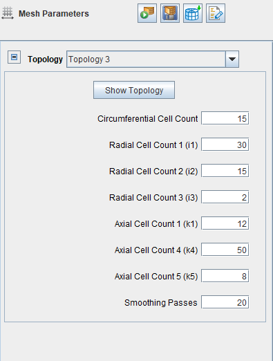
In the Mesh Controls > Remeshing Editor panel, the Smooth check box is unchecked. All other controls are left at default values.
On the Models > Chemistry/Materials Editor panel, the Diesel_2comp_189sp__soot-particle-tracking.cks chemistry set has been selected.
This chemistry set includes a gas-phase mechanism (Diesel_2comp_189sp__soot-particle-tracking_chem.inp), and a surface mechanism file (surf_soot_chem.inp). The thermodynamic data are included in the mechanism files.
The gas-phase mechanism contains 189 species participating in 1392 reactions. This mechanism has been generated for use with the 66.8/33.2 wt% n-decane/AMN diesel surrogate. It has reaction pathways to accurately predict soot precursors needed for the surface soot mechanism, all the way from small hydrocarbons such as acetylene to polycyclic aromatic species such as pyrene and coronene.
If you were to create your own chemistry set for use with particle tracking, the surface mechanisms would have to conform to certain standards, as defined in the Chemkin Input Manual and Chemkin Theory Manual. The soot surface mechanism that is part of this tutorial's chemistry set includes:
Soot nucleation through multiple pathways.
HACA- and PAH-based soot growth pathways.
Soot oxidation through O2 and OH.
The default values are used in the Transport property panel. In the Transport > Turbulence panel, the RANS RNG k-epsilon model is used, with default values.
Under Models > Spray model, the spray models, nozzle and fuel injection values have been set.
The nozzle-1 settings are provided in Table 6.3: Nozzle settings.
Table 6.3: Nozzle settings
|
Location |
|
|---|---|
|
Reference frame |
Global origin |
|
Coordinate system |
Cylindrical |
|
R |
0.1 cm |
|
q |
22.5 degrees |
|
A |
9 cm |
|
Spray direction
| |
|
Reference frame |
Global origin |
|
Coordinate system |
Spherical |
|
q |
110 degrees |
|
f |
22.5 degrees |
|
Nozzle size |
|
|
Nozzle diameter |
150 micron |
The following spray models are being used in this project, with default Ansys Forte settings:
KH droplet breakup model
RT droplet breakup model
Gas-jet
Vaporization model
Adaptive Collision Mesh droplet collision model
The diesel fuel was simulated using a 2-component surrogate consisting ([1]) of 66.8 weight% n-decane/33.2 weight% 1-methylnaphthalene. This particular surrogate was designed to model a European diesel fuel with cetane number of 55. This surrogate has a threshold sooting index of 36, placing it on the higher end of the typical diesel fuel sooting index. Table 6.4: Details of nozzle (Nozzle-1) and fuel injection (Injection-1) provides details of the nozzle and the fuel injection. These values are entered under the Models > Solid Injector-1 node. Specifically, the nozzle location and spray direction inputs are set on the Nozzle-1 Editor panel, and the fuel injection-related inputs are specified on the Injection-1 Editor panel.
On the Solid Injector-1 panel, parcel specification has been set using the Number of parcels option. The Injected parcel count has been set to 30,000.
The Inflow Droplet Temperature has been set to 320 K.
Spray was initialized using the Constant Discharge Coefficient and Angle option. A Discharge Coefficient of 0.9 has been used, with a Mean Cone Angle of 15°.
Table 6.4: Details of nozzle (Nozzle-1) and fuel injection (Injection-1)
|
Nozzle details |
|
|---|---|
|
Direct-injector nozzle hole |
150 μm |
|
Fuel injection details
| |
|
Start of injection (° ATDC) |
-10 |
|
Duration of injection (°) |
10 |
|
Total Injected mass (mg) |
20 |
|
Injection velocity profile |
A slightly modified square profile: (0,0), (1E-7,1), (0.999999,1), (1,0) |
Under Models > Soot Model, choose Soot Model. There are three options for modeling soot in Ansys Forte. One option is to define a "pseudo-gas" soot model that is included in a different gas-phase chemistry mechanism input. In that case, you would not select Models > Soot Model. With the selected chemistry in this example, you may either:
Use a built-in 2-step model, which is one option on the Soot Model panel.
Use the Method of Moments. This option enables the particle tracking capability. In this tutorial, Method of Moments is selected.
With the Method of Moments option selected in the Soot Model panel, four inputs are required. Details regarding these parameters can be found in the Chemkin Theory Manual.
Number of Moments: 3-6 moments can be used in the simulations. Typically, it is recommended that 3 moments are sufficient; that value of 3 is used in this tutorial.
Scaling Factor for Moments: This value changes the units of the (internal) solution variable for particle moments. A recommended value for typical problems is the default 1.0E+12, as the scaling helps preserve the positivity of the solution during computation.
Scaling Factor for Surface Species: This value changes the units of the (internal) solution variable for particle surface species. For example, setting it to 1.0E+12 results in pico-moles, while a value of 1 would mean that the unit should be moles. A recommended value for typical problems is the default 1.0E+12, as the scaling helps preserve the positivity of the solution during numerical computation.
Coagulation is included in this tutorial, with a Coagulation Collision Efficiency of 1.0. This coagulation collision efficiency term is a combined correction factor to the coalescent collision between particles. The van der Waals forces can enhance the collision frequency while non-coalescent collision can reduce the frequency.
Piston: The piston temperature is set to 500 K. The Law of the Wall model is used. Under Wall motion, the Bore is set to 9 cm and Stroke is set to 8 cm, and the Connecting Rod Length is set to 15 cm.
Periodicity: The Sector Angle is set to 45°.
Head: The Temperature is set to 470 K, and the Law of the Wall model is used.
Liner: The Temperature is set to 420 K, and the Law of the Wall model is used.
An ~10% EGR case is considered here. This results in an initial composition with a mass fraction of:
O2=0.2055
N2=0.7611
CO2=0.0246
H2O=0.0088
The initial Temperature and Pressure are set to values of 340 K and 2.0 bar. The initial Turbulent Kinetic Energy is set to 10,000 cm2/sec2, and the Turbulent Length Scale = 1 cm. Under Velocity, Engine Swirl is chosen and an Initial Swirl Ratio of 1.0 is used. The Initial Swirl Profile factor is left at the default value of 3.11. The Piston item is selected as the Piston Boundary.
The simulation Start Crank Angle (that is, Initial Crank Angle, under Simulation Controls in the Workflow tree) is set to -130 degrees ATDC, the Engine Speed is specified as 2000 RPM, and the simulation Final Simulation Crank Angle is set to +130 degrees ATDC.
To allow visualizing fuel and soot precursor species, the following species have been named in the Spatially Resolved and Spatially Averaged And Spray Output Control Editor panel. Also included in the list are species for air, combustion products, co, no, and no2.
Coronene (species name coronene)
Pyrene (species name a4)
Acenaphthalene (species name a2r5)
Naphthalene (species name naph)
Benzene (species name c6h6)
Phenyl (species name c6h5)
Acetylene (species name c2h2)
n-Decane, a fuel surrogate nc10h22
AMN, a fuel surrogate a2ch3
The spatially resolved values are output at (a) uniform intervals of 50 crank angle degrees, and (b) user-defined crank angle outputs at 0. 10, 20, 30, 40, and 50 crank angle degrees. The spatially averaged values are output every 0.5 crank angle degrees.
Spatially averaged plots appear below first, followed by some spatially resolved plots. The spatially resolved plots have been generated using EnSight.
The simulation results for the pressure and heat release rate are shown in Figure 6.2: Calculated pressure and apparent heat release rate curves. The fuel ignites slightly before TDC.
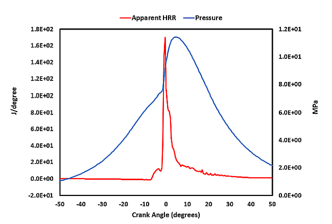
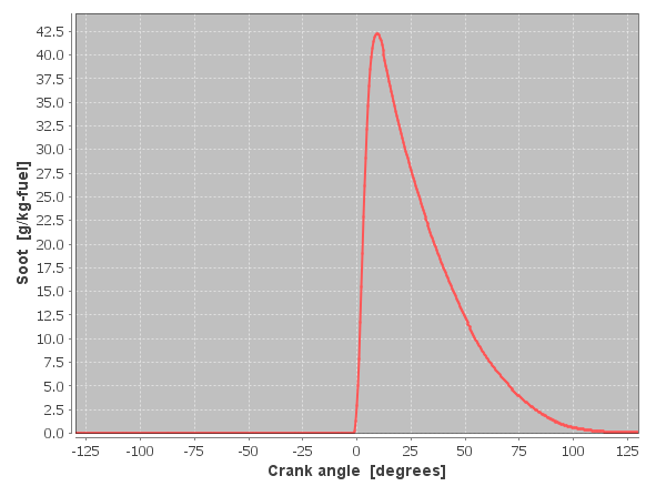
Figure 6.3: Predicted spatially averaged soot as a function of crank angle shows a line plot of the spatially averaged soot values, as a function of crank angle. Soot surface chemistry causes soot production, and soot reaches a maximum value of ~42.5 g/kg-fuel at ~10 CA degrees ATDC. Following this, the soot value decreases due to oxidation reactions to a value of 0.1 gm/kg-fuel at EVO (130 CA degrees ATDC). In addition to soot chemistry (multiple pathways for particle nucleation, growth, and oxidation), soot particle coagulation has also been accounted for in the simulations.
Next, we look at spatially resolved plots to understand more details of the soot evolution inside the engine. Spatially resolved plots have been generated using Ansys EnSight. Several soot particle outputs are potentially available to visualize, and a few of them are shown in this section.
Figure 6.4: A 2000K temperature isosurface showing the region of combustion at TDC (the cut plane shown here is used to plot values in the next figure) shows spatially-resolved values at TDC. Spray is nearing its end around this time, and ignition has occurred. The isosurface shown is that of 2000K temperature. A cut plane near the middle (25 deg theta) has been used to further understand soot evolution, and values are shown in this cut plane in the next figure, Figure 6.4: A 2000K temperature isosurface showing the region of combustion at TDC (the cut plane shown here is used to plot values in the next figure).
Figure 6.4: A 2000K temperature isosurface showing the region of combustion at TDC (the cut plane shown here is used to plot values in the next figure)
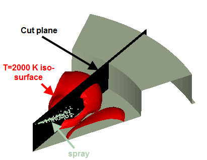
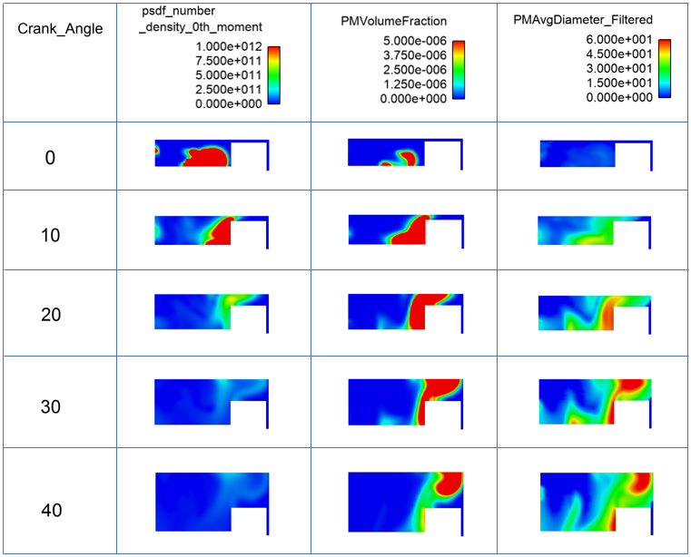
Figure 6.5: Soot particle number density (#particles/cm3), volume fraction (cm3/cm3) and average diameter (nm) shown on the cut plane from 0-40 CA degree ATDC uses iso-surfaces (50 nm) to show the spatially resolved values of average particle diameter, at 30-70 crank angle degrees. Of the three crank angles explored here, the 20 nm particles peak at 50 CAD, and the location of these relatively large particles is in the squish zone.
In Figure 6.5: Soot particle number density (#particles/cm3), volume fraction (cm3/cm3) and average diameter (nm) shown on the cut plane from 0-40 CA degree ATDC, the soot particle number density, volume fraction and average diameter are shown on the cut plane described above, for 0-40 CA degree ATDC. The following trends are seen:
When soot first starts to form near TDC, the particle number density is largest, and the average particle diameter is smallest. With time, the number density starts to go down, due to particle coagulation and due to particle consumption through oxidation. Meanwhile, the particle diameter starts to go up with time, up to 30-40 CA ATDC, because of coagulation and particle growth reactions. With more time (not shown here), the particle diameter starts to go down due to particle consumption through oxidation.
Particle volume fraction is highest in the 10-20 CA range.
Soot initially starts to form in the piston bowl, but eventually most of the soot is seen in the squish region.
Figure 6.5: Soot particle number density (#particles/cm3), volume fraction (cm3/cm3) and average diameter (nm) shown on the cut plane from 0-40 CA degree ATDC
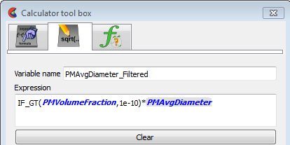
Note that the particle diameter shown in Figure 6.6: Filter used in EnSight for average particle diameter is a filtered value. Even when soot volume fraction is very low (say, less than 1E-10), the average diameter can potentially be a large value. However, in this scenario, the average particle diameter does not have much meaning as it is essentially due to numerical noise. To filter these kinds of values, the filtering shown in Figure 6.6: Filter used in EnSight for average particle diameter has been used. This filter shows only particle diameter when the local particle volume fraction is greater than 1E-10.
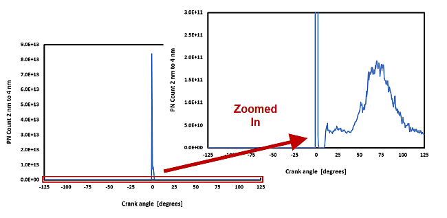
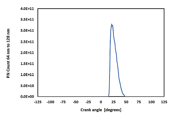
Finally, we show another option to analyze soot results. A file named ‘particle_size_distribution.csv’ is reported in the results directory when using soot Method of Moments in Forte. This file contains information on the particle number count for various ‘bins’ of particle sizes, and can be visualized in either the Forte Monitor. Figure 6.7: Particle number count reported for various particle binsshows some examples of the particle number counts. The first figure shows a spike around TDC, when soot is starting to form; this is probably from the nucleation reaction creating a lot of small particles, which subsequently grows to larger particles either because of coagulation or growth reactions. From 20 CA ATDC, a zoomed in version of the same plot shows that 2-4 nm particles again start to be formed, which could be either due to particle nucleation creating new particles, or particle destruction through oxidation resulting in formation of these size particles from larger particles. Also shown are particles from 64-128 nm, which start to form in substantial numbers around 20 CA, but are mostly consumed by 50 CA.
Figure 6.7: Particle number count reported for various particle bins shows the average particle size distribution. It can be seen that initially at 5-10 CAD, the particle count is high but the particle size is low with the majority of particles being smaller than 4 nm. With increasing crank angle, the lower, zoomed-in plot shows that larger diameter particles form but have lower particle count.