Post-Analysis allows you to view, compare, and post-process any case or data files located in or imported to the project.
Note: Post-Analysis makes use of the EnSight post-processing functionality and is directly displayed in the Fluent Aero workspace window.
This feature includes some important limitations to be aware of:
Using Post-Analysis with Fluent Solution files (.dat.h5) will display some surface variables as unavailable, and large solutions may have a long loading time.
Some Post-Analysis operations will not be recorded as journal commands, such as the reorientation of the Graphics window.
Complex Scenes and Viewports may not update completely in some scenarios.
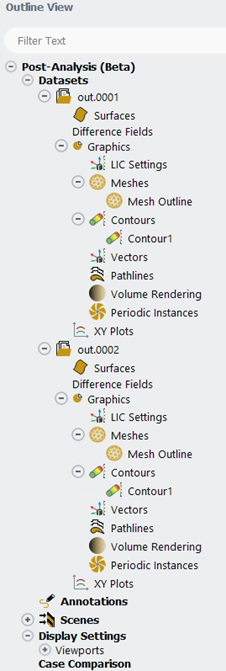
When the Post-Analysis feature is first activated, a Post-Analysis node will appear in the Outline View where detailed post-processing can be performed. In general, it can be used to create more custom post-processing objects or obtain more detailed solution data than what is otherwise available from the quick post-processing objects available in the Results node of a simulation.
Note: The Post-Analysis feature uses the EnSight renderer, therefore, the EnSight package must be included in the Ansys installation to use this feature inside Fluent Aero.
The following section gives some information on Post-Analysis commands that are available in Fluent Aero. For more detailed information on Post-Analysis, see Fluent Post-Analysis Workspace.
Datasets can be loaded into the Post-Analysis tool in two ways:
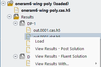
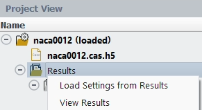
In the Project View, select a DP folder or solution file and choose or .
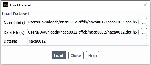
From the Results ribbon, select Dataset → . Browse to and select a matching case file and data file.
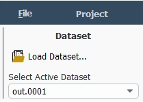
The current dataset can be selected through the Dataset menu or through a selection in the Outline View.
Note: Datasets marked with the prefix Fluent : refer to the currently active dataset associated with the currently loaded simulation, and are not loaded in the Post-Analysis viewer.
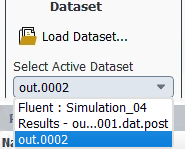
In the example shown in the images below, two datasets are currently loaded into the Post-Analysis tool: Results – out.0002 (which was loaded by selecting on the DP2 folder in the Project View) using the Project View and out.0001 (which was loaded using the command in the Results ribbon).
The Dataset entry will update as a specific dataset is highlighted in the Post-Analysis area of the Outline View, or if the Results node of a simulation is selected. Each additional dataset loaded to Post-Analysis is loaded using the same background EnSight instance, and will consume additional memory.
The following commands are available when left-clicking a Dataset name:
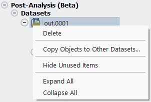
Datasets can be released and unloaded through the command. All graphical objects related to this dataset and its Scene entries will be removed.
This command enables you to copy the state of one dataset to another, including its list of graphical objects and their settings. This enables easy dataset comparison, especially if each dataset is shown in a separate viewport.
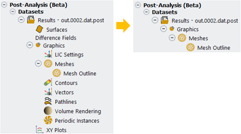
This command enables you to hide unused graphics objects in the list. For example, if only a Mesh object has been created, will reduce the list of objects under the dataset to show only the Meshes object. This can be helpful to reduce visual clutter when working with many datasets. Selecting will reveal the unused hidden objects.
The following graphics display control icons are available at the left side of the Post-Analysis graphics window:
 Set Layout
This menu can be used to split the graphics window into multiple viewports
 Set Active Viewport
This menu can be used to select the active viewport for graphical operations. Alternatively, the display or addition to a specific viewport can be set from the contextual menu on the graphical item by choosing →
 Link Viewports
This menu is used to synchronize the camera angles and movements of all viewports
Alternatively, the display or the addition of the selected graphical object to a specific viewport can be set from the contextual menu on the graphical item:
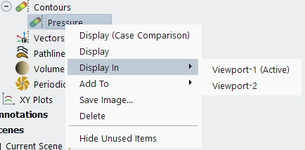
Displays the graphics object for the selected datasets side-by-side, in the Graphics window using the viewport layout specified under the Case Comparison node.
Displays the graphics object for the selected datasets in the Graphics window.
Displays the selected Graphics object within the viewport.
Adds the selected Graphics object to the viewport.
Opens the Save Picture dialog box allowing you to save an image file of the object in the Graphics window.
Deletes the selected Graphics object.
For quick access to commonly used commands, a context-sensitive menu is available when right-clicking within the Graphics window:
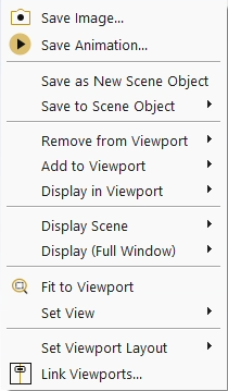
Opens the Save Picture dialog box allowing you to save an image file of the object in the Graphics window.
Opens the Save Animation dialog box allowing you to save an animation file.
Note: This setting is active only for transient datasets.
Saves the Graphics window content as an object under Scenes.
Saves the Graphics window content to an existing Scene object.
Adds the selected Graphics object to the viewport.
Displays the selected Graphics object within the viewport.
Removes the selected Graphics object from the viewport.
Displays the selected Scene object in the viewport.
Displays your model to take maximum advantage of the Graphics window’s width and height.
Adjusts the overall size of your model to take maximum advantage of the viewport’s width and height.
Contains a drop-down of views, allowing you to display the model from the direction of the vector equidistant to all three axes, as well as in different axes orientations.
Allows you to select from a collection of viewport arrangements.
Synchronizes the display of the selected viewports.
Each loaded dataset will have the following graphical objects available in Post-Analysis:
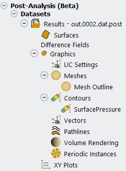
Surfaces
Generate new geometric surfaces or lines which can be used as selected surface zones when creating a Meshes, Contours or Vectors.
Difference Fields
Generate objects to display the difference of certain data fields.
Graphics
LIC Settings
Integrate a vector over a part surface to provide a uniform visualization of the flow of a vector over a surface.
Meshes
Generate mesh objects to display all or part of the mesh.
Contours
Generate colored contour plots of solution variables contained in the solution file.
Vectors
Generate vector plots of directional variables contained in the solution file.
Pathlines
Generate pathlines along surfaces using directional variables in the solution file.
Volume Rendering
Draw vectors in the entire domain, or on selected surfaces. By default, one vector is drawn at the center of each cell (or at the center of each facet of a data surface), with the length and color of the arrows representing the velocity magnitude. The spacing, size, and coloring of the arrows can be modified, along with several other vector plot settings.
Periodic Instances
Generate periodic instances objects to display repeated periodic surfaces.
XY Plots
Generate XY plots of solution data along 1D objects in the domain.
Note: To generate XY Plots, it is first required to generate a 1D graphical object on from the XY plot can collect its data. You can use Surface → New → Line… to generate an arbitrary line in the volume. Alternatively, you can use Surfaces → → to create a line resulting from the intersection of a list of surfaces. To do this, create an Iso-Surface on a coordinate Iso-Value, and , as shown in the image below:
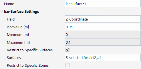
In this example, a Z cutting plane is selected at the middle of the domain and restricted to the walls of the domain, leading to a line along the airfoil surface where solution variables may be obtained for an XY Plot.
Mirror Planes
Create 2D XY plots of your results for analyzing one variable with respect to another variable. For more details on Mirror Planes, see Mirror Planes.
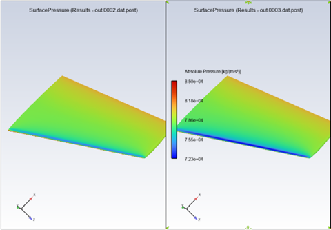
When multiple results can be loaded into Post-Analysis concurrently, the Case Comparison feature can be used to easily create side by side comparisons of different datasets.
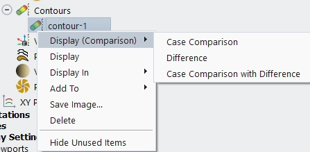
When more than one dataset is loaded into Post-Analysis, create a graphics object, for example a contour, in one of the datasets. Right-click that object and select . The graphics object will automatically be copied to all datasets, and the Scenes → Current Scene will be automatically adjusted such that the graphics window will display a side-by-side comparison of the datasets.
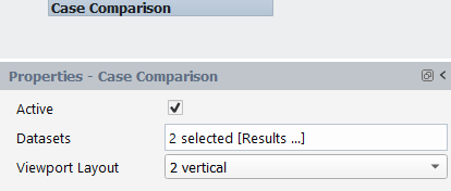
A maximum of 4 datasets will be displayed at a time. The Case Comparison object can be used to adjust datasets that are currently selected.
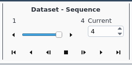
The entire sequence of design point solutions can be loaded by selecting the Results folder in the Project View and choosing .
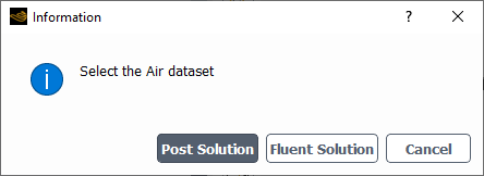
Depending on which solution files are available, the command will offer a choice to load either the Post Solution or the Fluent Solution. In general, it is preferred to load the Post Solution, as these files contain selected variables and are quicker to load into Post-Analysis.
When a full results folder’s sequence of design point solutions is loaded into Post-Analysis, the Dataset – Sequence ribbon section permits you to change the currently displayed item in the sequence.