


This technique models the effect of the rotor on the flow field in a time-averaged manner through momentum equation source terms placed in a disk volume swept by the spinning rotor. Two tasks must be addressed simultaneously in this approach:
Time-averaged solution of the flow field through and around the rotor.
Reduced-order solution of the rotor blade aerodynamics to compute the required momentum source terms.
In our approach for the first task, the flow field is solved using Ansys Fluent, inviscid or viscous laminar or turbulent simulations can be obtained, assuming that the fluid is either compressible or incompressible. The following is, therefore, an outline of our approach to the formulation and implementation of task 2.
The momentum source terms, unknown at the start of the simulations, are linked to the flow solution through the actuator disks and therefore evolve as part of the iterative solution. The momentum source terms are evaluated using the Blade Element Theory by replacing the rotor blades with a stack of airfoil sections in the spanwise direction. Each section is treated as if it were a 2D airfoil. The geometric properties of each section, such as chord length, airfoil type and twist can vary along the span of the blade.
In typical CFD simulations, rotorcraft are assumed to be stationary and immersed in a
moving airstream, hence airflow solutions around rotorcraft are computed in the absolute
frame of reference. Since the blades are rotating around an axis with velocity
 , they are best described in a relative frame of reference defined by
their rotation axis and origin, the radial direction along the blade and the azimuthal
angle that defines the position of the blade in its circle of rotation. In VBM
simulations, a third local 2D frame of reference is needed, defined by the tangential
velocity vector at the blade section and the normal vector of the rotor disk. In order
to compute the forces acting on a blade section, it is necessary to transform the
velocity field
, they are best described in a relative frame of reference defined by
their rotation axis and origin, the radial direction along the blade and the azimuthal
angle that defines the position of the blade in its circle of rotation. In VBM
simulations, a third local 2D frame of reference is needed, defined by the tangential
velocity vector at the blade section and the normal vector of the rotor disk. In order
to compute the forces acting on a blade section, it is necessary to transform the
velocity field  computed in the absolute frame of reference to the local blade section
frame of reference to obtain the relative velocity field, from which the local angle of
attack (α), Mach number (
computed in the absolute frame of reference to the local blade section
frame of reference to obtain the relative velocity field, from which the local angle of
attack (α), Mach number ( ), and Reynolds number (
 ), can be determined. Look-up tables corresponding to each blade
section are then used to extract the local
), can be determined. Look-up tables corresponding to each blade
section are then used to extract the local  and
and  values, from which the instantaneous rotor forces per unit rotor span
can be computed in the form:
values, from which the instantaneous rotor forces per unit rotor span
can be computed in the form:

where  is the chord length as a function of the non-dimensional radius
  ,
,  is the rotor tip radius and
  is the instantaneous relative airflow velocity experienced by each
blade cross-section in the frame of reference of the rotor. However, for the
time-averaged solution in the absolute frame of reference, these forces must be
time-averaged over one rotation. Assuming that the rotational speed is constant, time
averaging over one period is identical to geometric averaging over an angle
is the instantaneous relative airflow velocity experienced by each
blade cross-section in the frame of reference of the rotor. However, for the
time-averaged solution in the absolute frame of reference, these forces must be
time-averaged over one rotation. Assuming that the rotational speed is constant, time
averaging over one period is identical to geometric averaging over an angle
 . Therefore, the time-averaged forces on a cell with face area
 on the rotor disk becomes:

where  is the number of blades, and
  is the radial coordinate of cell center.
The above force vector  is transformed back into the absolute flow field reference frame
vector
is transformed back into the absolute flow field reference frame
vector  so that it can be included in the airflow calculation. Let
  be the cell volume, then:

is the time-averaged source term per unit volume that is added to the momentum equations in every cell attached to the rotor disk. Once these source terms have been computed, the solution of the flow field can be obtained, and the iterative procedure is repeated until the convergence criteria are met. This generalized implementation supports both structured and hybrid unstructured mesh topologies with hexahedral and prismatic elements.
The rotor performance is controlled by the thrust and moment coefficients, which are defined as:

where  = 1 in North American (NA) practice and
  = ½ in European practice. In NA practice, the coefficient ½
is absorbed into the thrust and moment coefficients, whereas in European practice the
formulae explicitly contains the coefficient ½, therefore
= ½ in European practice. In NA practice, the coefficient ½
is absorbed into the thrust and moment coefficients, whereas in European practice the
formulae explicitly contains the coefficient ½, therefore

In Fluent VBM,  is set to 1.
Finally, a comment should be made regarding turbulence modeling. CFD solvers such as
Ansys Fluent employ a wide range of turbulence models to account for the
effects of turbulence on the mean flow for steady-state fluid flow simulations. For
applications where the VBM is used, it is suggested that standard two equation models
such as  or
or  be employed. It should be noted that the VBM itself does not affect
the turbulence model directly by increasing the production of turbulence kinetic energy
within the modeled rotor zone. However, turbulent mixing is modeled downstream of the
VBM rotor zones, and therefore turbulence is indirectly influenced by the momentum
generated by the rotors.
be employed. It should be noted that the VBM itself does not affect
the turbulence model directly by increasing the production of turbulence kinetic energy
within the modeled rotor zone. However, turbulent mixing is modeled downstream of the
VBM rotor zones, and therefore turbulence is indirectly influenced by the momentum
generated by the rotors.
Fluent VBM replaces the rotor system with momentum sources acting on a layer of cells for each rotor zone. These cells can be created in the mesh as a one-cell-thick actuator disk, called Embedded Disk method (EDM), or can be searched in the mesh when cut by a disk surface geometry, called Floating Disk method (FDM).
If using EDM, an internal surface in the shape of a flat disk should be created in the flow domain at the location of the rotor. In the CAD, this surface should be marked as an internal wall or internal surface that will be discretized by a single layer of nodes, such that the mesh is continuous across the surface. A single uniform layer of prisms or hexahedral cells should be extruded from the cell faces attached to the disk in the direction normal to the disk. The prismatic layer of cells in the downstream of the disk should be marked as a separate cell zone such that each rotor has its own separate cell zone. When calculating the airflow, Fluent VBM reads cells of each zone in a loop and calculate the source terms. Creating a mesh with these criteria would be difficult specially for a case with many rotors. However, it will provide more accurate and stable results. In addition, for unsteady simulation in this mode, any movement of disk requires mesh displacement or replacement which is not practical.
When using FDM, there is no need to create rotor disks and corresponding prismatic layers in the mesh. Instead, you only create a mesh with any type of element around the fuselage or any bodies in the domain without considering the rotor disk. The floating disk can be created using the post-processing tools available in Fluent to create a plane surface and clip it by iso-clip, or it can be imprinted as a .stl file. In VBM's Graphical User Interface (GUI), you can simply set up the disk center, orientation, and tip and root radius, and press a button to create the floating disk. Meshing Guidelines and Creating the VBM Disk explains the mesh guidelines and how to define and create the floating disk in the mesh.
The current implementation of the VBM allows a maximum of twenty-five rotor disks. This enables the simulation of complex rotorcraft with multiple rotors, from simple helicopters with main and tail rotor, to multiple tilt rotors, to quadcopters and even to multiple rotorcraft, and single- or multi-engine propeller aircraft. It also can be used to simulate airflow around wind turbines in a large wind farm.
The rotor disk geometry is characterized by the location of its center {X,Y,Z}, its tip and root radius and its pitch and bank angles (or the rotor disk normal vector) as shown in Figure 18.1: Rotor Disks Schematic.
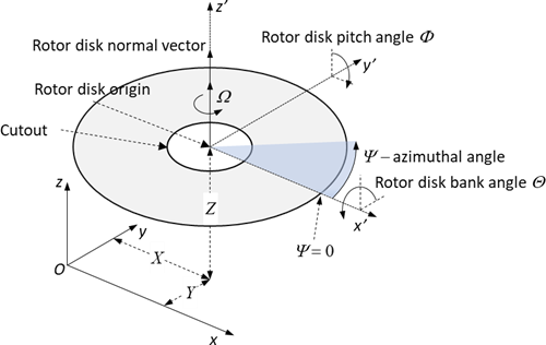
In the current implementation of VBM, the natural orientation of the disk’s
normal vector points in the positive Z-direction.
Should the orientation of the normal vector be different, the disk must be rotated
from its natural orientation first by using the disk pitch angle  (rotation around the Y-axis) and then bank angle
  (rotation around the x’-axis
  ). Therefore, when a pitch rotation is applied, the x’-axis of the rotor will no longer be parallel to
the X-axis.
). Therefore, when a pitch rotation is applied, the x’-axis of the rotor will no longer be parallel to
the X-axis.
Note:
Rotations are not additive.
Rotations are non-commutative and must be applied consistently in this order.
Rotations follow the right-hand rule.
This also applies to the inclination of the rotor during CAD construction −
the rotations must be applied in the same order. For example, in the case of an
aircraft equipped with a propeller whose normal axis is aligned in the negative
X-direction, the pitch and bank angles must be
set to  = −90˚,
  = 0˚. Similarly, if the rotor axis is aligned in the
positive Y-direction, the pitch and bank angles
should be set to
= 0˚. Similarly, if the rotor axis is aligned in the
positive Y-direction, the pitch and bank angles
should be set to  = 0˚,
= 0˚,  = -90˚.
Rotor disk position can also be set using disk normal vector components instead of disk pitch and bank angles. In that case, Fluent’s VBM computes disk pitch and bank angles according to the above mentioned natural orientation and disk normal vector.
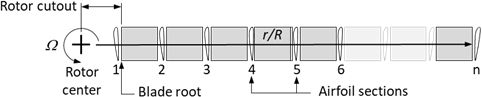
The blades are represented as stacks of airfoils which can vary in chord, twist
and airfoil type along the normalized blade span  , as shown in Figure 18.2: 3D Blade Geometry Represented by a Stack of 2D Airfoils. The VBM
assumes a linear distribution of chord, twist and
, as shown in Figure 18.2: 3D Blade Geometry Represented by a Stack of 2D Airfoils. The VBM
assumes a linear distribution of chord, twist and  and
and  between the two ends of each section. Simulation accuracy
increases if the airfoil look-up tables contain data for a range of Reynolds (
between the two ends of each section. Simulation accuracy
increases if the airfoil look-up tables contain data for a range of Reynolds ( ) and Mach numbers (
 ) covering all possible operating conditions, since the VBM can
determine the local
) covering all possible operating conditions, since the VBM can
determine the local  and
and  on the blade and interpolate
  and
and  from the tables accordingly.
The blade pitch angle q(y), not to be confused with the rotor pitch angle, is the angle of the
blade with respect to the rotor disk plane. To a first-order approximation
(neglecting blade torsional flexing and other harmonics), it consists of the
baseline collective angle  and a cyclic pitch component expressed as a function of the sine
and cosine of the azimuthal angle
and a cyclic pitch component expressed as a function of the sine
and cosine of the azimuthal angle  :
:

The blade pitch angles  ,
,  , and
, and  can either be prescribed by you or calculated by the automatic
rotor trim routine. The collective angle
can either be prescribed by you or calculated by the automatic
rotor trim routine. The collective angle  is the angle of the blade at some point on its span with respect
to the disk surface. The angles
is the angle of the blade at some point on its span with respect
to the disk surface. The angles  and
and  , the amplitudes of the cosine and sine components of the cyclic
pitch, are directly related to the angles of the swash plate found on most
helicopter rotors and therefore control the pitch and roll attitude of the
rotorcraft. Most rotor/propeller blades also have a spanwise twist. The blade twist
adds to the collective pitch, therefore, reference point for the collective pitch
and twist angles can be defined arbitrarily at any position along the blade as long
as their sum provides correct rotor pitch angle. Traditionally, for helicopters, the
reference point for the twist is located at 3-quarters of the blade span, therefore,
helicopter main rotors usually have negative twist towards the tip. Negative twist
progressively reduces the angle of attack towards the tip, increases the stall and
buffeting margins, unloads the outer blade region and increases flapping
stability.
, the amplitudes of the cosine and sine components of the cyclic
pitch, are directly related to the angles of the swash plate found on most
helicopter rotors and therefore control the pitch and roll attitude of the
rotorcraft. Most rotor/propeller blades also have a spanwise twist. The blade twist
adds to the collective pitch, therefore, reference point for the collective pitch
and twist angles can be defined arbitrarily at any position along the blade as long
as their sum provides correct rotor pitch angle. Traditionally, for helicopters, the
reference point for the twist is located at 3-quarters of the blade span, therefore,
helicopter main rotors usually have negative twist towards the tip. Negative twist
progressively reduces the angle of attack towards the tip, increases the stall and
buffeting margins, unloads the outer blade region and increases flapping
stability.
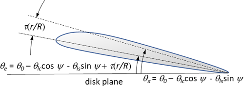
The VBM saves the effective pitch angle over the entire rotor as one of several VBM data fields in the solution file. The effective pitch angle is defined as:

where  is the twist angle as a function of the normalized radius, as
shown in Figure 18.3: Effective Pitch Angle as a Function of r/R and
is the twist angle as a function of the normalized radius, as
shown in Figure 18.3: Effective Pitch Angle as a Function of r/R and  .
.
Articulated helicopter rotor blades can flap in response to the centrifugal and
aerodynamic forces they endure. The flapping motion is not computed by the model,
however, if the characteristics of the flapping motion is known, the model can
account for the rotor coning angle and the first flapping harmonics by transforming
the velocity components from the rotor disk plane to the actual tip path plane.
Therefore, the baseline coning angle  and the longitudinal and lateral flapping coefficients
 and
and  determine the resultant flapping angle:
  :
:

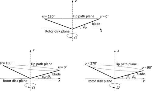
Figure 18.4: Blade Flapping – Baseline β0 (Top), Longitudinal and Lateral Components β1c, β1s (Bottom) shows a schematic of the flapping blades in the x-z and y-z planes.
Note: The disk of the rotor remains flat and the flapping of the blades is simulated.
Figure 18.4: Blade Flapping – Baseline β0 (Top), Longitudinal and Lateral Components β1c, β1s (Bottom)
The change in the angle of attack due to flapping is computed, however the
relatively small flapping velocity component  that should be added to the velocity component normal to the blade
path is neglected. Furthermore, due to its relatively small effect, the lead-lag
motion of the blade is neglected.
that should be added to the velocity component normal to the blade
path is neglected. Furthermore, due to its relatively small effect, the lead-lag
motion of the blade is neglected.
The rotors of helicopters operating in forward flight generate asymmetrical load distributions with respect to the plane defined by the forward velocity vector and the rotor normal vector. In addition to the collective pitch control required to maintain level flight at the desired altitude, cyclic pitch is necessary to balance the load across the rotor and control the pitching and rolling moments. Accurate aerodynamic simulations are only possible when the rotors are operating at the desired thrust and pitching/rolling moment settings. These settings, however, must be transformed into rotor blade pitch angles - a non-trivial operation. An automatic trim routine is available to compute the correct rotor settings without costly empirical guesswork. Thrust and moments with respect to the center of the rotor can be formulated in terms of non-dimensional thrust and moment coefficients.
Rotorcraft


Propeller


where  is the rotor tip speed and
  is the aircraft forward speed.
Since rotorcrafts in hover have no forward velocity, the dynamic pressure must be formulated in terms of the rotor tip speed, whereas for propellers the aircraft forward speed is normally used.
Important: In Fluent VBM, the thrust and moment coefficients are defined as functions of the rotor tip speed for both propellers and rotors.
The reference area of the rotor  is defined solely by its tip radius
  and includes the disc cutout, or the spinner cutout in the case of
a propeller.
and includes the disc cutout, or the spinner cutout in the case of
a propeller.
The VBM trimming routine calculates the collective and cyclic pitch angles to achieve the desired thrust and pitching (y-axis) and rolling (x-axis) moments around the hub. Let the three coefficients be expressed as functions of the collective and cyclic angles:

Note: The effect of the flapping hinge offset is neglected in the calculation of the moments.
Since the relationship between the rotor aerodynamic parameters and the blade
pitch is non-linear, an iterative technique is used to drive the trim procedure to
convergence. Following Yang et al. (References), a
Newton-Raphson iterative method is employed to automatically trim any number of
rotors in the computational domain to achieve the user-set target values
 .
.
The simulation begins with a user-supplied initial guess for the angles
 of each rotor
  . After every
  airflow iterations, called update frequency, the flow solver
pauses and the VBM computes the rotor parameters
airflow iterations, called update frequency, the flow solver
pauses and the VBM computes the rotor parameters  . A new set of angles is computed for each rotor i with the Newton-Raphson iterative approach. Let

The system of equations can be solved easily by recasting it in the form

With initial angles  The angles are updated as follows

where  is a tunable under-relaxation factor, such that
  . The recommended value is 0.8.
The VBM then recomputes the source terms and the flow solution resumes. Since there are no analytical equations for computing the coefficients of the Jacobian matrix, the derivatives are obtained in the frozen flow field at time level n by computing the thrust and moment coefficients after perturbing each angle independently by the amount ±a. For example, the first coefficient, representing the derivative of the thrust coefficient with respect to the collective angle, would be approximated by

Since the derivatives are computed numerically, the algorithm is really the Secant
Method. This procedure is repeated at every N iterations, until the rotor
performance parameters reach their target values and the flow solution is converged.
The L2 norms of  ,
,  and
and  are computed and printed on the Fluent
Console to show the convergence of the trimming routine. The
trimming routine is robust and yields converged results for cases simulating
multiple rotors.
are computed and printed on the Fluent
Console to show the convergence of the trimming routine. The
trimming routine is robust and yields converged results for cases simulating
multiple rotors.
Rotor blades usually have very high aspect ratios, therefore the lift and drag forces can be computed to a reasonable approximation at each spanwise location by assuming two-dimensional flow. However, near the tip, the circulation around the blade induced by the lift force is turned by 90˚ and shed downstream. The turning of the circulation creates the tip vortex, which introduces lift and drag losses that the VBM is unable to model directly.
To obtain a more realistic solution, the tip loss effects are incorporated in VBM
using a tip loss factor  that corrects lift and drag coefficients near the tip of the disk,
such that:
that corrects lift and drag coefficients near the tip of the disk,
such that:


where the lift/drag coefficient  /
/ is interpolated in airfoil data tables based on the
 at the cell centroid of each element on the disk. Since drag
coefficient cannot be lower than the minimum drag coefficient for any airfoil,
corrected drag coefficient is enforced to be above this number.
at the cell centroid of each element on the disk. Since drag
coefficient cannot be lower than the minimum drag coefficient for any airfoil,
corrected drag coefficient is enforced to be above this number.

Two options are available in VBM to calculate the tip loss factor as follows:
Quadratic Tip Loss Function: Using this option, tip losses are approximated by a damping function inversely proportional to the square of the distance to the blade tip, starting from a user-specified radial threshold, named tip loss limit
 (default set at 96% of the rotor span
  ).
).Modified Prandtl’s Tip Loss Function: Prandtl’s tip loss function is generally used in Blade Element Momentum Theory (BEMT) that equates two set of equations of the momentum balance on a rotating annular stream tube passing on a disk (momentum theory, or MT) and the forces acting on the blade element at the corresponding sections along the blade span (blade element theory or BET). In VBM, however, Reynolds-averaged Navier–Stokes equations (RANS) and BET are applied such that RANS can capture the tip loss effects near the tip of rotor disk. However, that does not represent the tip loss near the tip of the actual rotor. Therefore, a modified version of this function is used in VBM such that you can tune it for each application. In VBM, the tip loss factor
 is calculated using:
 where
 is the tuning coefficient and
  is given in terms of the number of the blades
  , the radial position of blade element
  , the rotor radius
  , and induced inflow angle
  , defined as the angle between the normal and tangential
components of relative incident velocity at each blade section where an
element exists.
, defined as the angle between the normal and tangential
components of relative incident velocity at each blade section where an
element exists.The tuning coefficient
 should be larger than 1, set by you in the VBM user
interface.
should be larger than 1, set by you in the VBM user
interface.


