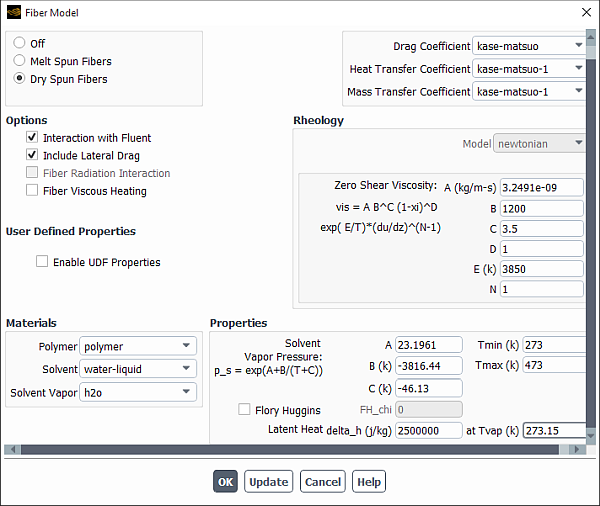
With Ansys Fluent’s fiber model, you can model two types of fibers: melt spun and dry spun. The model you choose depends on the polymer that is used to draw the fibers. If the fiber polymer can be molten without being destroyed thermally, then a melt spun fiber process is typically used to produce the fibers. In such cases, select Melt Spun Fibers under Model in the Fiber Model dialog box (Figure 34.1: The Fiber Model Dialog Box).

When the fiber polymer can be liquefied with a suitable solvent, or the fiber polymer’s production process involves a solvent, the fibers are formed typically in a dry spinning process. In such cases, select Dry Spun Fibers under Model in the Fiber Model dialog box (Figure 34.1: The Fiber Model Dialog Box).

If the fibers in your simulation strongly influence the flow of the surrounding fluid and need to be considered, you must select Interaction with Fluent under Options in the Fiber Model dialog box (Figure 34.1: The Fiber Model Dialog Box). When iterating a solution with Ansys Fluent, the fiber model equations are solved alternating with Ansys Fluent’s flow equations. Source terms are also computed to couple the fiber equations with the fluid flow equations. The calculation of the source terms is performed only during the course of an Ansys Fluent computation. See Coupling Between Fibers and the Surrounding Fluid for a description of the source terms.

In typical fiber simulations, the axial drag of the fibers is the most important force acting on the fibers as well as on the surrounding fluid. In some situations, the lateral or cross-flow drag can become important. This is the case when the fibers are mainly cooled or dried in a cross-flow situation. In such cases you can select Include Lateral Drag under Options in the Fiber Model dialog box (Figure 34.1: The Fiber Model Dialog Box). The drag is estimated for a cylinder in cross-flow and is shown in Equation 22–30. Lateral drag is not considered by the fiber equations and therefore lateral bending of the fibers is not considered.

In some situations radiative heat exchange is important. If you are using Ansys Fluent’s P-1 radiation model or Ansys Fluent’s discrete ordinates (DO) radiation model, you can consider the effects of irradiation on the cooling and heating of the fibers. When you are using the DO radiation model, the effects of the fibers upon the DO model can be considered. If the DO radiation model is enabled, you can select Fiber Radiation Interaction (Options group box) and enter the fiber’s Emissivity in the Properties group box (see Figure 34.1: The Fiber Model Dialog Box).

When high elongational drawing rates are combined with large fiber viscosities, viscous heating of fibers may become important. To consider this effect in the fiber energy equation (Equation 22–12), you can select Fiber Viscous Heating under Options in the Fiber Model dialog box (Figure 34.1: The Fiber Model Dialog Box).

The effects of the boundary layer of the fiber are modeled in terms of drag, heat transfer, and mass transfer coefficients. These parameters are specified under Exchange in the Fiber Model dialog box (Figure 34.1: The Fiber Model Dialog Box).