


Conservation equations for momentum, mass, and energy for individual parcels in the wall-film are described below. The particle-based approach for thin films was first formulated by O’Rourke [495] and most of the following derivation is based closely on that work.
The equation for the momentum of a parcel in the film is:
 | (12–270) |
|
where | |
 = is the film particle velocity = is the film particle velocity | |
 = is the magnitude of the shear stress of the gas
flow on the surface of the film = is the magnitude of the shear stress of the gas
flow on the surface of the film | |
 = is the unit vector in the direction of the film surface velocity = is the unit vector in the direction of the film surface velocity | |
 = is the stress that the wall exerts on
the film = is the stress that the wall exerts on
the film | |
 = is the force per unit area necessary to keep the film on the surface = is the force per unit area necessary to keep the film on the surface | |
 = is the current film height
at the particle location = is the current film height
at the particle location | |
 = is the
body force term = is the
body force term |
Despite the small values of film thickness, the body force term can be very significant due to the very high acceleration rates seen in simulations with moving boundaries.
The expression for the wall stress,  , is:
, is:
 | (12–271) |
where  is the liquid film
viscosity and
is the liquid film
viscosity and  is the wall velocity.
The force  is included in Equation 12–270 for completeness, but
is not modeled in the formulation of the equations solved in Fluent. Instead, it is accounted
for by explicitly enforcing the condition:
is included in Equation 12–270 for completeness, but
is not modeled in the formulation of the equations solved in Fluent. Instead, it is accounted
for by explicitly enforcing the condition:
 | (12–272) |
at each time step for all particles representing the wall-film.
Ansys Fluent solves a particle position equation of the form:
 | (12–273) |
After rearranging Equation 12–270 and substituting Equation 12–271 the film particle acceleration is given by:
 | (12–274) |
The film vaporization law is applied when the film particle temperature is above the
vaporization temperature  . In Ansys Fluent, the vaporization rate is modeled using following models:
Diffusion Controlled Model
Convection/Diffusion Controlled Model
Gas-Side Boundary Layer Model
Film Boiling Model
The film vaporization rate is governed by gradient diffusion from the surface exposed to the gas phase. The gradient of vapor concentration between the film surface and the gas phase is
 | (12–275) |
where  is the molar flux of vapor (kmol/m2-s),
 is the mass transfer coefficient (m/s), and
  and
and  are the vapor concentrations on the film surface and in the bulk gas,
respectively (kmol/m3).
are the vapor concentrations on the film surface and in the bulk gas,
respectively (kmol/m3).
The vapor concentration at the film surface is evaluated using the saturated vapor pressure at the film temperature, and the bulk gas concentration is obtained from the flow field solution. The vaporization rate is sensitive to the saturated vapor pressure, similar to the droplet vaporization.
The film mass transfer coefficient is obtained as:
(12–276) |
where  is the binary diffusivity of species
  ,
,  is the Nusselt correlation, and the
  is the characteristic length (in meters) computed as the square root of the
film parcel area
is the characteristic length (in meters) computed as the square root of the
film parcel area  :
:
 | (12–277) |
 is taken to be a mass weighted percentage of the wall face area
 :
:
 | (12–278) |
In Equation 12–276 for the mass transfer coefficient, the Nusselt correlation is used after replacing the Prandtl number with the Schmidt number as follows:


where the Reynolds number  is calculated from the particle film characteristic length
  and the particle relative velocity component that is parallel to the
wall.
and the particle relative velocity component that is parallel to the
wall.
For multicomponent vaporization, the diffusivity of each species is used in Equation 12–276 and Equation 12–279 to obtain the vaporization rate of each component in the liquid film mixture.
The mass of the particle parcel  is decreased according to:
 | (12–281) |
where  is the molecular weight of the gas phase species
  to which the vapor from the liquid is added. The diameter of the film
particle is decreased to account for the mass loss in the individual parcel. This keeps the
number of drops in the parcel constant.
to which the vapor from the liquid is added. The diameter of the film
particle is decreased to account for the mass loss in the individual parcel. This keeps the
number of drops in the parcel constant.
The film vaporization rate is governed by:
 | (12–282) |

|
where | |
|
| |
|
| |
|
| |
|
|


The single-rate thermolysis model uses Equation 12–87 and the
constant rate model uses Equation 12–88. If the Lagrangian wall film is
considered, the secondary rate model that allows you to differentiate between the thermolysis
rates of free-stream particles and film particles can be applied. The model uses Equation 12–87 to calculate separately the mass transfer rate from the free
particle to the bulk gas phase (using the particle pre-exponential factor  and the particle activation energy
  ) and the mass transfer rate from the film to the bulk gas phase (using the
film pre-exponential factor
) and the mass transfer rate from the film to the bulk gas phase (using the
film pre-exponential factor  and the film activation energy
  ).
).
When the partial pressure of species in the bulk is less than the vapor pressure at the film surface, Fluent uses Equation 12–291 and Equation 12–292 to calculate the vaporization rate for laminar and turbulent flows, respectively. The equations are using wall functions to determine the mass transfer coefficients. See Film Condensation for details.
When the film temperature reaches the boiling point, the film boiling rate is calculated
by setting the right-hand side of the energy balance equation (Equation 12–301) to 0 in and solving for the film boiling
rate  .
.
The resulting boiling rate expressions are as follows:
Constant Temperature Walls
 | (12–283) |
Heat Flux Walls
 | (12–284) |
with:
 | (12–285) |

|
where | |
|
| |
|
| |
|
| |
|
| |
|
| |
|
| |
|
| |
|
| |
|
|


If the Gas-Side Boundary Layer model is enabled, the heat transfer coefficient
 is computed as follows.
Laminar flow:
 , where the length
  is the normal distance from film surface to the bulk.
Turbulent flow:
 is determined from the wall functions as described in Energy Transfer from the Film.
In other cases, Fluent uses the Nusselt number expression:
 | (12–286) |
|
where | |
|
| |
|
|


The Nusselt number  is computed from Equation 12–299. If the film is
cooled below the boiling point by contacting a cold wall, the vaporization rate calculation
will revert to the vaporization equations (Equation 12–275 or Equation 12–282).
is computed from Equation 12–299. If the film is
cooled below the boiling point by contacting a cold wall, the vaporization rate calculation
will revert to the vaporization equations (Equation 12–275 or Equation 12–282).
The boiling rate expressions for the convective heat transfer model are as follows:
For constant temperature walls:
 | (12–287) |
For heat flux walls:
 | (12–288) |
with
 | (12–289) |
In the above equations,
 = mass of the film particle (kg) = mass of the film particle (kg) |
 = film particle temperature (K) = film particle temperature (K) |
 = bulk temperature (K) = bulk temperature (K) |
 = wall temperature (K) = wall temperature (K) |
 = latent heat of vaporization (J/kg) = latent heat of vaporization (J/kg) |
 = heat transfer coefficient from wall to liquid film
(W/K-m2) = heat transfer coefficient from wall to liquid film
(W/K-m2) |
 = heat transfer coefficient from liquid film to bulk phase
(W/K-m2) = heat transfer coefficient from liquid film to bulk phase
(W/K-m2) |
 = film parcel area, taken to be a mass weighted percentage of the wall face
area (m2) = film parcel area, taken to be a mass weighted percentage of the wall face
area (m2) |
 = heat flux imposed on the wall (W) = heat flux imposed on the wall (W) |
 = liquid Prandtl number = liquid Prandtl number  |
The heat transfer coefficient from liquid film to bulk phase ( ) is obtained as described in Film Boiling Model with Conduction Heat Transfer Model.
The heat transfer coefficient from wall to liquid film  is obtained from Equation 12–312.
If the film is cooled below the boiling point by contacting a cold wall, the vaporization rate calculation will revert to the vaporization equations (Equation 12–275 or Equation 12–282).
The condensation model is triggered when the partial pressure of species  in the bulk exceeds its vapor pressure at the film surface. The Fluent Lagrangian wall film model uses two different expressions for wall film condensation under laminar and turbulent flow conditions. The derivation follows [739], assuming that the condensation of species
  from the gas phase takes place in the presence of noncondensables.
In the Ansys Fluent Lagrangian Wall Film Condensation model, component  condenses on the wall film in the presence of non-condensable components. For the condensation rate of component
  through a plane at a distance
  from the film surface, Fick’s law can be written as:
 | (12–290) |
|
where | |
|
| |
|
| |
|
| |
|
|


For laminar flow, the mass fraction of species  is integrated from the film surface to the bulk gas conditions yielding the logarithmic term, while in case of turbulent flow, finite differences are taken directly. The final expressions are:


|
where | |
|
| |
|
|


For laminar flow, the mass transfer coefficient  in Equation 12–291 is computed as:
 | (12–293) |
where  is the normal distance from the film surface to the bulk.
  is computed as the normal distance from the wall adjacent cell center to the wall.
For turbulent flow, the turbulent mass transfer coefficient  in Equation 12–292 is determined from the wall functions. The current implementation uses wall functions as described by Equation 4–348. When the enhanced wall treatment is enabled in the turbulence model, the implementation follows the calculations in Enhanced Wall Treatment ε-Equation (EWT-ε).
For multicomponent particles, Equation 12–291 or Equation 12–292 are applied to each liquid component.
See Film Condensation Model in the Fluent User's Guide for more information on how to use the film condensation model.
For the multicomponent Lagrangian wall film, the vaporization rate is calculated as the sum of the vaporization rates of the individual components. The vaporization rate of each component in the liquid film are computed from:
Diffusion Controlled model: Equation 12–275 and Equation 12–276
Convection/Diffusion Controlled model: Equation 12–282
If the Thermolysis model has been enabled for any component in the film, Ansys Fluent applies Equation 12–164 to obtain the thermolysis rate of the individual component for the single rate or Equation 12–165 to obtain the constant rate.
If the Lagrangian wall film is considered, the secondary rate model can be used. This
model uses Equation 12–164 to calculate separately the vaporization rate of
the free-stream particle (using the particle pre-exponential factor and the particle activation energy ) and the vaporization rate of the film (using the film pre-exponential factor
and the film activation energy ).
When the total vapor pressure at the multicomponent film surface exceeds the cell
pressure, Ansys Fluent applies a multicomponent film boiling equation by using averaged forms of
Equation 12–283 or Equation 12–284 in
accordance with the thermal boundary condition applied at the wall. The average latent heat
 is computed according to Equation 12–170 from the latent
heats of the individual liquid components and the overall boiling rate of the film is
calculated by averaging the rates computed from Equation 12–283 or
Equation 12–284 for the conduction heat transfer model, and from
Equation 12–287 or Equation 12–288 for the convective
heat transfer model, for each liquid component for each liquid component with the fractional
vaporization computed by Equation 12–171.
is computed according to Equation 12–170 from the latent
heats of the individual liquid components and the overall boiling rate of the film is
calculated by averaging the rates computed from Equation 12–283 or
Equation 12–284 for the conduction heat transfer model, and from
Equation 12–287 or Equation 12–288 for the convective
heat transfer model, for each liquid component for each liquid component with the fractional
vaporization computed by Equation 12–171.
To obtain an equation for the temperature in the film, energy flux from the gas side as well as energy flux from the wall side must be considered. In the absence of film evaporation/boiling, the energy transfer from/to the film particle is then given by:
 | (12–294) |
|
where | |
|
| |
|
| |
|
|


When the thermal boundary condition on the wall is set to a constant temperature,
 is calculated as:
 | (12–295) |
|
where | |
|
| |
|
| |
|
|


For walls where the heat flux,  is imposed by the boundary condition, Equation 12–295 is replaced by:
 | (12–296) |
The convective heat flux,  , is calculated as:
 | (12–297) |
|
where | |
|
| |
|
|


If the film condensation or the gas-side boundary layer model is enabled, the heat
transfer coefficient  is computed as follows.
Laminar flow:

(12–298)
where
 is the normal distance from the film surface to the bulk.
  is computed as the normal distance from the wall adjacent cell center to
the wall.
is computed as the normal distance from the wall adjacent cell center to
the wall.Turbulent flow:
 is determined from the wall functions. The current implementation uses wall
functions as de- scribed in Standard Wall Functions, Equation 4–343. When the enhanced wall treatment is enabled in the
turbulence model, the implementation follows the calculations in Enhanced Wall Treatment ε-Equation (EWT-ε)
is determined from the wall functions. The current implementation uses wall
functions as de- scribed in Standard Wall Functions, Equation 4–343. When the enhanced wall treatment is enabled in the
turbulence model, the implementation follows the calculations in Enhanced Wall Treatment ε-Equation (EWT-ε)
In other cases, Fluent uses a Nusselt number expression for  :
:

|
where | |
|
| |
|
|


The Nusselt number  is calculated as:
 | (12–299) |
The film surface temperature  in Equation 12–297 is determined from the
interface conservation relation:
in Equation 12–297 is determined from the
interface conservation relation:
 | (12–300) |
When the particle changes its mass during vaporization, an additional term is added to Equation 12–294 to account for the enthalpy of vaporization:
 | (12–301) |
where  is the film parcel vaporization rate (kg/s), and
  is the latent heat of vaporization (J/kg).
As the film parcel trajectory is computed, Ansys Fluent integrates Equation 12–294 or Equation 12–301 and obtains the temperature at the next time step.
The implementation does not account for film radiation effects. The energy source terms are calculated for the film parcels from the energy difference along the film trajectory. For the cases where the film resides on a wall with heat-flux imposed, the heat losses or gains from the film to the wall equal the heat-flux values. For all other thermal boundary conditions, except heat flux, Fluent determines the film temperature based on the wall temperature and the heat transferred from the bulk fluid to the film. The total heat flux to the wall is then calculated by adding the heat flux from the bulk fluid to the wall and the heat flux from the film to the wall.
The convective wall-film heat transfer model provides a more accurate calculation of heat transfer between the Lagrangian wall film and the wall surface where it is formed. It is especially useful for thicker wall films, films moving at high velocity and where the film liquid material has a high Prandtl number. Refer to Setting the Lagrangian Wall Film Model in the Fluent User's Guide to learn how to use this model.
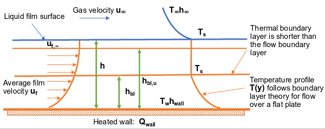
The following assumptions are made for the flow and heat transfer in the liquid film:
The film flow is laminar.
The velocity and temperature profiles in the liquid film follow the laminar boundary-layer theory for flow over a flat plate as described in [372].
The velocity boundary layer
 is located above the thermal boundary layer
  .
. For film heights significantly lower than the thermal boundary layer, the heat transfer reverts to pure conduction.
The film is always in complete contact with the wall.
The energy balance of a film particle at temperature  exchanging heat with a wall surface and a bulk phase can be expressed
as:
exchanging heat with a wall surface and a bulk phase can be expressed
as:
 | (12–302) |
with
 | (12–303) |
and
 | (12–304) |
where
 = mass of the film particle (kg) = mass of the film particle (kg) |
 = heat capacity of the liquid (J/K-kg) = heat capacity of the liquid (J/K-kg) |
 = film particle temperature (K) = film particle temperature (K) |
 = latent heat of vaporization (J/kg) = latent heat of vaporization (J/kg) |
 = heat transfer coefficient from wall to liquid film
(W/K-m2) = heat transfer coefficient from wall to liquid film
(W/K-m2) |
 = heat transfer coefficient from liquid film to bulk phase
(W/K-m2) = heat transfer coefficient from liquid film to bulk phase
(W/K-m2) |
 = wall face area (m2) = wall face area (m2) |
 = film parcel area, taken to be a mass weighted percentage of the wall face
area = film parcel area, taken to be a mass weighted percentage of the wall face
area  (m2) (m2) |
 = bulk temperature (K) = bulk temperature (K) |
 = film surface temperature (K) = film surface temperature (K) |
 = wall temperature (K) = wall temperature (K) |
 = heat flux imposed on the wall (W) = heat flux imposed on the wall (W) |
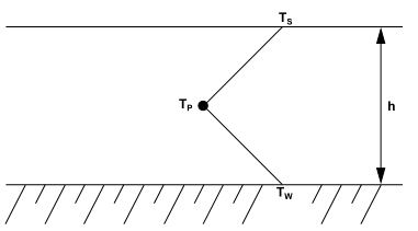
The temperature profile inside the thermal boundary layer in the direction  normal to the wall is expressed as:
 | (12–305) |
where  is the boundary layer height.
The film temperature above the thermal boundary remains constant at  .
.
The average temperature inside the boundary layer  can be obtained by integrating along the
  direction:
 | (12–306) |
which results in:
 | (12–307) |
The average film parcel temperature  can be obtained by weighting
  and
and  with the heights
  and (
and ( ) under the assumptions that the film velocity and density remain
constant:
) under the assumptions that the film velocity and density remain
constant:
 | (12–308) |
where  is the liquid film height.
For  > 0.6, the ratio of the thermal boundary layer thickness to the velocity
boundary layer thickness can be represented as:
> 0.6, the ratio of the thermal boundary layer thickness to the velocity
boundary layer thickness can be represented as:
 | (12–309) |
The surface temperature  can be calculated by combining equations Equation 12–307 -
Equation 12–309 for the constant temperature walls:
can be calculated by combining equations Equation 12–307 -
Equation 12–309 for the constant temperature walls:
 | (12–310) |
For walls where the constant heat flux  is imposed, the corresponding equation for the surface temperature is
expressed as:
is imposed, the corresponding equation for the surface temperature is
expressed as:
 | (12–311) |
As the film parcel trajectory is computed, Ansys Fluent integrates Equation 12–302 and obtains the temperature at the next time step.
The model implementation does not account for film radiation effects. The energy source terms are calculated for the film parcels from the energy difference along the film trajectory. For cases where the film resides on a wall with heat-flux imposed, the heat losses or gains from the film to the wall equal the heat-flux values. For all other thermal boundary conditions, except heat flux, Ansys Fluent determines the film temperature based on the wall temperature and the heat transferred from the bulk fluid to the film. The total heat flux to the wall is then calculated from Equation 12–304 .
Calculation of the heat transfer coefficient 
The heat transfer coefficient from film to wall is expressed as:
 | (12–312) |
where  is the thermal conductivity of the liquid film, and
  is the characteristic length.
The Nusselt number  is calculated from the laminar boundary-layer theory for
  > 0.6:


In the above equations, the Reynolds number and the Prandtl number  are calculated as:
 | (12–315) |
 | (12–316) |
where
 , ,  , ,  , and , and  = density, viscosity, thermal conductivity and heat capacity of the liquid
film, respectively. = density, viscosity, thermal conductivity and heat capacity of the liquid
film, respectively. |
 = velocity of the liquid film in the bulk, that is, above the film flow
boundary layer (m/s) = velocity of the liquid film in the bulk, that is, above the film flow
boundary layer (m/s) |
Calculation of
The velocity profile for fully developed flow over a flat plate in the laminar boundary
layer is described in the direction normal to the wall by:
 | (12–317) |
The flow boundary layer height  can be obtained as function of distance
  from the edge of the flat plate [372]:
 | (12–318) |
The bulk velocity  is calculated as a function of the average wall film velocity
  for the following regimes:


Considerations on the characteristic length 
is the distance of the current particle location from the impingement point.
The impingement location is known for new film particles only and can only be recorded during
the impingement event. It cannot be back-calculated when reading film particles from case/data
files created in earlier versions. For those old particles, the film height is used as the
characteristic length  together with the below expressions for the Nusselt number
  providing the averaged heat transfer coefficients over a specified
length.
providing the averaged heat transfer coefficients over a specified
length.
The Nusselt number for  > 0.6 is expressed as:


Considerations on the heat transfer coefficient
The heat transfer coefficient  is computed by Equation 12–312 as a function of the
Nusselt number. However, it reverts to the conduction heat transfer coefficient
is computed by Equation 12–312 as a function of the
Nusselt number. However, it reverts to the conduction heat transfer coefficient  under the below conditions:
The Reynolds number is small, which may happen if the film velocity is low, or at the beginning of the film particle path
The film height is located well below the thermal boundary layer

In those cases, the temperature profile in the film is assumed to be linear, and the
characteristic length will be equal to the film height  .
.
The conduction heat transfer coefficient is computed as:
 | (12–322) |
Turbulent film approximation for heat transfer
For high film Reynolds numbers, the film-to-wall heat transfer is significantly enhanced because of turbulence phenomena. Ansys Fluent provides a simplified approach that improves the heat transfer predictions when the film is in the turbulent regime.
For the heat transfer calculations only, the following assumptions are made:
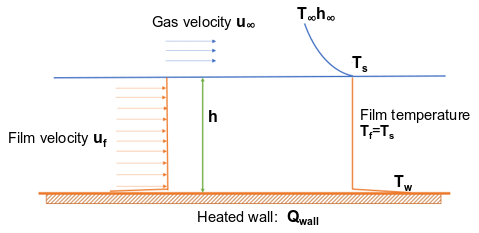
Both the transitional flow regime and the fully turbulent flow regime are defined based on the film local Reynolds number.
For the fully turbulent flow regime, both the velocity and temperature profiles in the film are flat (see Figure 12.15: Fully Turbulent Film Flow Regime: Velocity and Temperature Profile Assumptions ).
With the Reynolds number  expressed by
 | (12–323) |
where  is the film average velocity, and the remaining nomenclature is the same as
in Equation 12–315, the Nusselt number for the wall-to-film heat transfer is defined as follows:
is the film average velocity, and the remaining nomenclature is the same as
in Equation 12–315, the Nusselt number for the wall-to-film heat transfer is defined as follows:
Fully turbulent flow regime (
 ):
):
(12–324)

(12–325)
The flat temperature profile is achieved by setting
 in Equation 12–310 or Equation 12–311.
Transitional flow regime (
 ):
):The Nusselt number is defined as the largest of the
numbers computed by Equation 12–326 and either Equation 12–313 or Equation 12–321. The cubic temperature
profile assumption (Equation 12–305) is still maintained.
(12–326)
Here:

(12–327)
and

(12–328)
For the fully turbulent flow regime, the
number is set as the minimum of the values predicted by Equation 12–326 and Equation 12–324.The
 number limits have been calibrated with the data reported by
Åkesjö et al. [12] and [86]:
number limits have been calibrated with the data reported by
Åkesjö et al. [12] and [86]:

Calculation of the heat transfer coefficient from wall to film on the impingement point
The boundary layer theory is not applicable at the particle impingement point. Here, the
following expression for the Nusselt number is used [373]:
 | (12–329) |
Here, the Reynolds number is expressed as:
 | (12–330) |
where  is the jet velocity (m/s).
The characteristic length  used in the above expression is the jet diameter, which is approximated by
the reference diameter for the relevant injection type. The reference diameter is defined as
the hydraulic diameter corresponding to the surface area of the surface injection, or the
maximum particle diameter for injections involving particle size distributions.
used in the above expression is the jet diameter, which is approximated by
the reference diameter for the relevant injection type. The reference diameter is defined as
the hydraulic diameter corresponding to the surface area of the surface injection, or the
maximum particle diameter for injections involving particle size distributions.