At the center of the electrochemistry is the computation of the rates of the anodic and cathodic reactions. The electrochemistry model adopted in Ansys Fluent is one that has been used by other groups ([325], [419], and [663]).

The driving force behind these reactions is the surface overpotential: the difference between the phase potential of the solid and the phase potential of the electrolyte/membrane. Therefore, two potential equations are solved. One potential equation (Equation 20–3) accounts for the electron transport of through the solid conductive materials and is solved in the TPB catalyst layer, the solid grids of the porous media, and the current collector; the other potential equation (Equation 20–4) represents the protonic (that is, ionic) transport of and is solved in the TPB catalyst layer and the membrane. The two potential equations are as follows:

(20–3)

(20–4)

In the above equations, subscripts and refer to the membrane and solid phases, respectively.

The following figure illustrates the boundary conditions that are used to solve for and .

Figure 20.2: Boundary Conditions for the Electric Potentials (Solid and Membrane) — PEM Fuel Cell

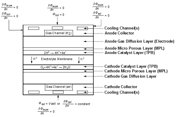
There are two types of external boundaries: those that have an electrical current passing through them, and those that do not.

As no ionic current leaves the fuel cell through any external boundary, there is a zero flux boundary condition for the membrane phase potential, , on all outside boundaries.

For the solid phase potential, , there are external boundaries on the anode and the cathode side that are in contact with the external electric circuit. Electrical current generated in the fuel cell only passes through these boundaries. On all other external boundaries there is a zero flux boundary condition for .

On the external contact boundaries, fixed values for (potentiostatic boundary conditions) are recommend. If the anode side is set to zero, the (positive) value prescribed on the cathode side is the cell voltage. Specifying a constant flux (say on the cathode side) means to specify galvanostatic boundary conditions.

The transfer currents, or the source terms in Equation 20–3 and Equation 20–4, are nonzero only inside the catalyst layers and are computed as:

The source terms in Equation 20–3 and Equation 20–4, also called the exchange current density (A/m³), have the following general definitions:

(20–5)

(20–6)

where
	= reference exchange current density per active surface area (A/m2)
	= specific active surface area (1/m)
	, = local species concentration, reference value (kmol/m3)
	= concentration dependence
	and = anode and cathode transfer coefficients of the anode electrode, respectively (dimensionless)
	and = anode and cathode transfer coefficients of the cathode electrode, respectively (dimensionless)
	= surface overpotential given by Equation 20–11
	= surface overpotential given by Equation 20–12
	= Faraday constant (9.65x107 C/kmol)
	= the universal gas constant
	= temperature

The above equation is the general formulation of the Butler-Volmer function. Note that the effects of the number of electrons in electrochemistry reactions are accounted for in the transfer coefficients. A simplification to this is the Tafel formulation given by:

(20–7)

(20–8)

By default, the Butler-Volmer function is used in the Ansys Fluent PEMFC model to compute the transfer currents inside the catalyst layers. When the magnitude of the surface over-potential () is large, the Butler-Volmer formulation reduces to the Tafel formulation.

In Equation 20–5 through Equation 20–8, and represent the molar concentration of the species upon which the anode and cathode reaction rates depend, respectively. That is, represents and represents .

The reference exchange current density and are dependent on the local temperature as follows:

(20–9)

(20–10)

The driving force for the kinetics is the local surface overpotential, , also known as the activation loss. It is generally the difference between the solid and membrane potentials, and .

(20–11)

(20–12)

The half cell potentials at anode and cathode and are computed by Nernst equations as follows [586]:

(20–13)

(20–14)

where is the water saturation pressure (Equation 20–54) and , , and are the partial pressures of hydrogen, oxygen, and water vapor, respectively. In the above equations, the standard state (, ), the reversible potentials and , and the reaction entropies and are user-specified quantities.

From Equation 20–3 through Equation 20–14, the two potential fields can be obtained.

 

20.1.2.1. The Cathode Particle Model

When Equation 20–8 is used to compute the cathode transfer current, the mass transport resistance in the catalyst microstructure is not considered ([586]). The resistance may consist of two parts:

• Resistance due to an ionomer film

• Resistance due to a liquid water film surrounding particles

In the Ansys Fluent PEMFC model, including these resistances in calculations of the transfer current is optional. The volumetric transfer current inside the cathode layers is represented by:

(20–15)

where is the concentration of oxygen at the wall. The is a user-specified value, and the is calculated by:

(20–16)

where
	= specific active surface area for the cathode catalyst (1/m)
	= liquid saturation
	= porosity
	= particle radius
	= product of oxygen solubility and diffusivity in liquid water (on the order of 10-10 m2/s)

The in Equation 20–15 is calculated as:

(20–17)

Here, is the ideal transfer current computed using Equation 20–6, but without considering resistance.