Chapter 1: Fluid Flow in an Exhaust Manifold

This tutorial is divided into the following sections:

1.1. Introduction

Note: This tutorial is fully supported at all licensing levels.

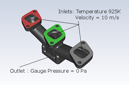
This tutorial illustrates the setup and solution of a three-dimensional turbulent fluid flow and heat transfer problem in a manifold. The manifold configuration is encountered in the automotive industry. It is often important to predict the flow field and temperature field in the area of the mixing region in order to properly design the junction.

This tutorial demonstrates how to do the following in Ansys Fluent:

Use the Watertight Geometry guided workflow to:
- Import a CAD geometry
- Generate a surface mesh
- Cap inlets and outlets
- Extract a fluid region
- Generate a volume mesh
Set up appropriate physics and boundary conditions.
Calculate a solution.
Review the results of the simulation.

Related video that demonstrates steps for setting up, solving, and postprocessing the solution results for a turbulent flow within a manifold:

1.2. Prerequisites

This tutorial is written with the assumption that you have completed the introductory tutorials found in this manual and that you are familiar with the Ansys Fluent outline view and ribbon structure. Some steps in the setup and solution procedure will not be shown explicitly.

1.3. Problem Description

The manifold modeled here is shown in Figure 1.1: Manifold Geometry for Flow Modeling. Hot air flows through the three inlets at 925 K and the same inlet velocity of 10 m/s, and then exits through the outlet. Convective heat transfer takes place between the fluid and the manifold.

Figure 1.1: Manifold Geometry for Flow Modeling

1.4. Setup and Solution

The following sections describe the setup and solution steps for this tutorial:

1.4.1. Preparation

To prepare for running this tutorial:

Download the exhaust_manifold.zip file here .
Unzip exhaust_manifold.zip to your working directory.
The SpaceClaim CAD file manifold.scdoc can be found in the folder. In addition, the manifold.pmdb file is available for use on the Linux platform.

1.4.2. Launching Ansys Fluent

From the Windows Start menu, select Start > Ansys 2024 R2 > Fluid Dynamics > Fluent 2024 R2 to start Fluent Launcher.
Fluent Launcher allows you to decide which version of Ansys Fluent you will use, based on your geometry and on your processing capabilities.
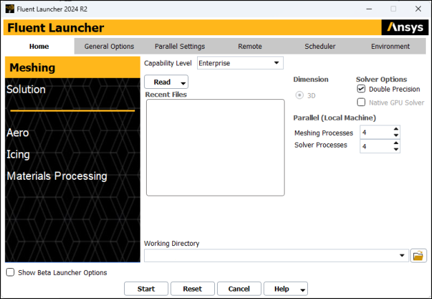
Ensure that the proper options are enabled.
1. Select Meshing in the top-left selection list to start Fluent in Meshing Mode.
2. Ensure that the Double Precision option is selected.
3. Set Processes to 4 under the Parallel (local Machine).
Note: Fluent will retain your preferences for future sessions.
Set the working folder to the one created when you unzipped manifold.zip.
1. Enter the path to your working folder for Working Directory by double-clicking the text box and typing.
  Alternatively, you can click the browse button ( ) next to the Working Directory text box and browse to the directory, using the Browse For Folder dialog box.
Click Start to launch Ansys Fluent.

1.4.3. Meshing Workflow

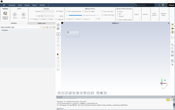
Start the meshing workflow.
1. In the Workflow tab, select the Watertight Geometry workflow.
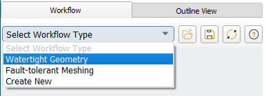
2. Review the tasks of the workflow.
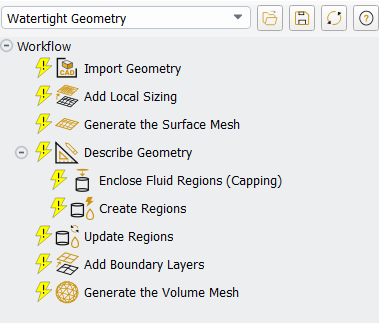
  Each task is designated with an icon indicating its state (for example, as complete, incomplete, etc. All tasks are initially incomplete and you proceed through the workflow completing all tasks. Additional tasks are also available for the workflow.
Import the CAD geometry (manifold.scdoc).
1. Select the Import Geometry task.
2. For File Format, keep the default setting of CAD.
3. For Units, keep the default setting as mm.
4. For File Name, enter the path and file name for the CAD geometry that you want to import (manifold.scdoc).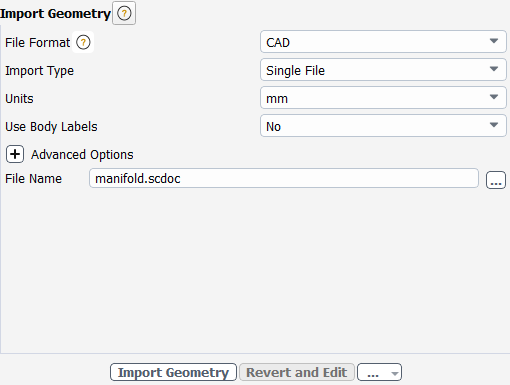
  Note: The workflow only supports *.scdoc (SpaceClaim), Workbench (.agdb), and the intermediary *.pmdb file formats.
5. Select Import Geometry.
  This will update the task, display the geometry in the graphics window, and allow you to proceed onto the next task in the workflow.
  Note: Alternatively, you can use the ... button next to File Name to locate the CAD geometry file, after which, the Import Geometry task automatically updates, displaying the geometry in the graphics window, and the workflow automatically progresses to the next task.
  Throughout the workflow, you are able to return to a task and change its settings using either the Edit button, or the Revert and Edit button.
Add local sizing.
1. In the Add Local Sizing task, you are prompted as to whether or not you would like to add local sizing controls to the faceted geometry.
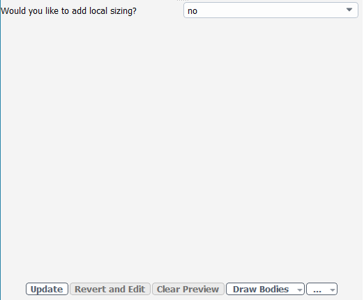
2. For the purposes of this tutorial, you can keep the default setting of no.
3. Click Update to complete this task and proceed to the next task in the workflow.
Generate the surface mesh.
1. In the Generate the Surface Mesh task, you can set various properties of the surface mesh for the faceted geometry.
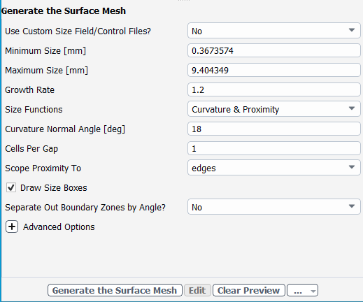
2. For the purposes of this tutorial, you can keep the default settings.
  Note: The red boxes displayed on the geometry in the graphics window are a graphical representation of size settings. These boxes change size as the values change, and they can be hidden by using the Clear Preview button.
3. Click Generate the Surface Mesh to complete this task and proceed to the next task in the workflow.
Describe the geometry.
When you select the Describe Geometry task, you are prompted with questions relating to the nature of the imported geometry.
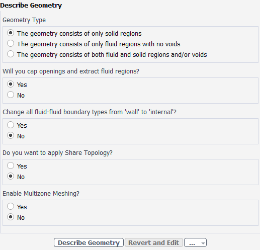
1. Since a fluid region is extracted from the solid model and capping surfaces are added, the default settings are appropriate.
2. Click Describe Geometry to complete this task and proceed to the next task in the workflow.
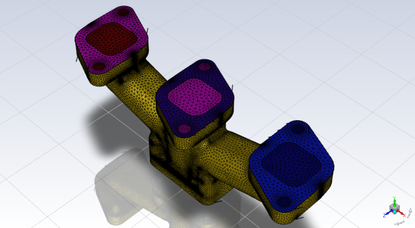
Cover any openings in your geometry.
Select the Enclose Fluid Regions (Capping) task where you can cover or cap any openings in your geometry in order to later extract the enclosed fluid region.
1. Create a cap for the inlets.
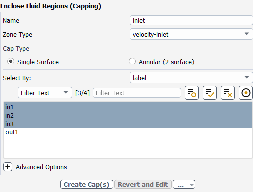
  1. In the Name field, assign a name for the capping surface (for example, inlet) to be assigned to all of the manifold's inlets.
  2. For the Zone Type, keep the default setting of velocity-inlet.
  3. For the Select By field, keep the default setting of label.
  4. In the list of labels, select in1, in2, and in3 for the openings that you want to cover.
    For occasions when the list of items is long, you can use the Filter Text option and use an expression such as in* to show only items starting with "in". Alternatively, you can use the Use Wildcard option to list and pres-select matching items. See Filtering Lists and Using Wildcards for more information.
    The graphics window indicates the selected items.
  5. Click Create Cap(s) to complete this task and proceed to the next task in the workflow.
2. Create a cap for the outlet.
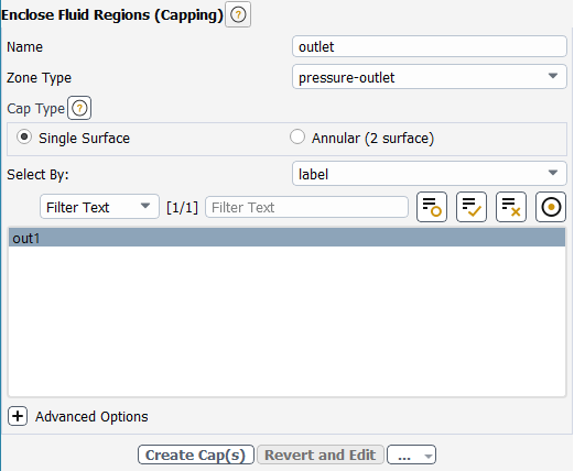
  1. In the Name field, assign a name for the capping surface (for example, outlet) to be assigned to the manifold's outlet.
  2. For the Zone Type, change the setting to pressure-outlet.
  3. For the Select By field, keep the default setting of label.
  4. In the list of labels, select out1 for the outlet that you want to cover.
  5. Click Create Cap(s) to complete this task.
  Now, all of the openings in the geometry are covered.
Create the fluid region.
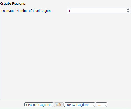
1. Select the Create Regions task, where you can determine the number of fluid regions that need to be extracted. Ansys Fluent attempts to determine the number of fluid regions to extract automatically.
2. For the Estimated Number of Fluid Regions, keep the default selection of 1.
3. Click Create Regions.
Update your regions.
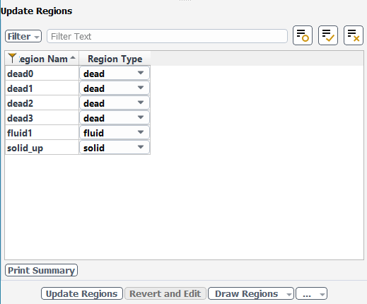
1. Select the Update Regions task, where you can review the names and types of the various regions that have been generated from your imported geometry, and change them as needed.
2. Keep the default settings, and click Update Regions.
  Aside from fluid regions and solid regions, you can also have voids within your geometry that are designated as dead regions. As you can see, there are four dead regions that correspond to the four bolt holes near the outlet, a solid region and a fluid region.
  Once the regions have been updated, the fluid region is displayed by default in the graphics window. You can use the Draw Regions button to display other options, such as drawing just the solid region, just the dead regions, or all regions.
Add boundary layers.
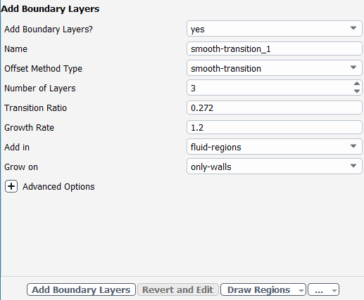
1. Select the Add Boundary Layers task, where you can set properties of the boundary layer mesh.
2. Keep the default settings, and click Add Boundary Layers.
Generate the volume mesh.
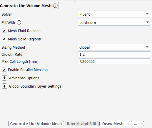
1. Select the Generate the Volume Mesh task, where you can set properties of the volume mesh.
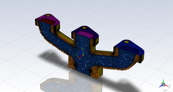
2. Keep the default settings, and click Generate the Volume Mesh.
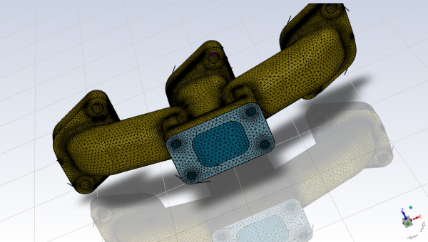
  Ansys Fluent will apply your settings and proceed to generate a volume mesh for the manifold geometry. Once complete, the mesh is displayed in the graphics window and a clipping plane is automatically inserted with a layer of cells drawn so that you can quickly see the details of the volume mesh.
Check the mesh.
Mesh → Check → Perform Mesh Check
Save the mesh file (manifold.msh.h5).
File → Write → Mesh...
Switch to Solution mode.
Now that a high-quality mesh has been generated using Ansys Fluent in meshing mode, you can now switch to solver mode to complete the set up of the simulation.
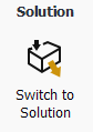
We have just checked the mesh, so select Yes when prompted to switch to solution mode.

1.4.4. General Settings

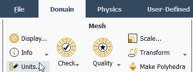
In the Mesh group box of the Domain ribbon tab, set the units for length..

Domain → Mesh → Units...

This opens the Set Units dialog box.

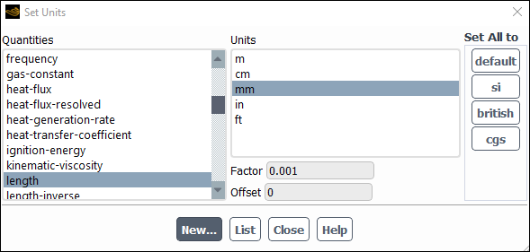
Select length under Quantities.
Select mm under Units.
Close the Set Units dialog box.

1.4.5. Solver Settings

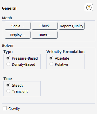
In the Solver group box of the Physics ribbon tab, retain the default selection of the steady pressure-based solver.

Physics → Solver → General

1.4.6. Models

Enable heat transfer by activating the energy equation.
Setup → Models → Energy On
Retain the default k-ω SST turbulence model.
You will use the default settings for the k-ω SST turbulence model, so you can enable it directly from the tree by right-clicking the Viscous node and choosing SST k-omega from the context menu.
Setup → Models → Viscous Model → SST k-omega

1.4.7. Materials

Change the default material of Aluminum to cast iron.

Create solid material properties for Cast Iron.
Setup → Materials → Solid → aluminum Edit...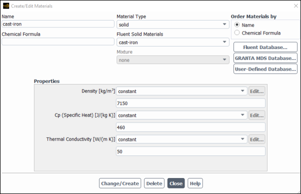
1. Change the name of the material to be cast-iron.
2. Clear the Chemical Formula field.
3. Change the Density to 7150 kg/m³.
4. Change the Cp to 460 J/kg K.
5. Change the Thermal Conductivity to 50 W/(m-K).
6. Click Change/Create and overwrite the aluminum material.
7. Click Yes to replace the aluminum material.
8. Close the Create/Edit Materials dialog box.

1.4.8. Cell Zone Conditions

Ordinarily, you would set up the cell zone conditions for the CFD simulation using the Zones group box of the Physics ribbon tab.

The properties of air for the fluid zone and cast-iron for the solid zone will be used.

1.4.9. Boundary Conditions

Set the velocity, turbulence, and thermal boundary conditions for the first inlet (inlet).
Setup → Boundary Conditions → Inlet → inlet Edit...
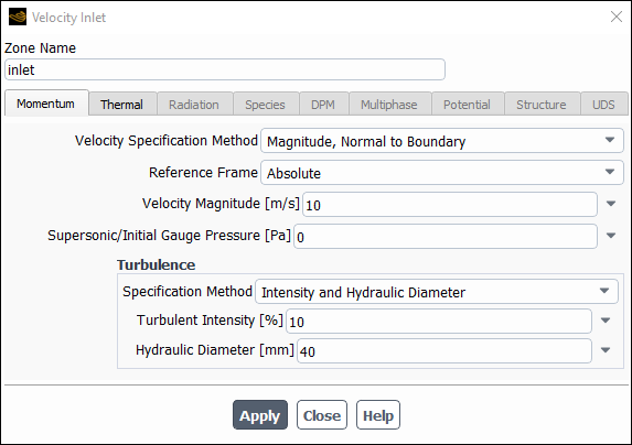
1. Enter 10 m/s for Velocity Magnitude.
2. In the Turbulence group box, select Intensity and Hydraulic Diameter from the Specification Method drop-down list.
3. Enter 10 % for the Turbulent Intensity.
4. Enter 40 mm for the Hydraulic Diameter.
5. Click the Thermal tab
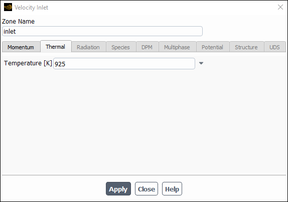
6. Enter 925 [K].
7. Click Apply and close the Velocity Inlet dialog box.
Apply the same conditions to the other inlets (inlet1, and inlet2).
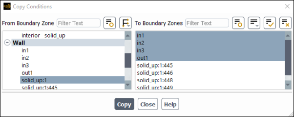
1. Select inlet from the Boundary Conditions node of the Outline View, right-click and select Copy from the context menu.
  This opens the Copy Conditions dialog box.
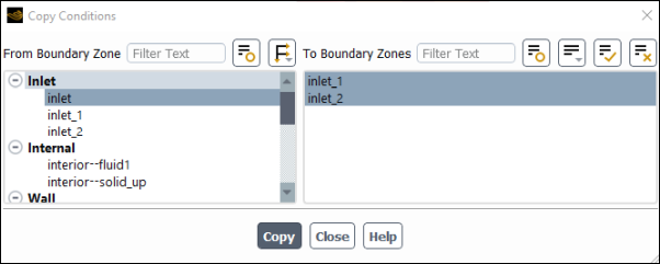
2. Select inlet _1 and inlet_2 from the To Boundary Zones list.
3. Click Copy, click OK in the confirmation prompt, and close the Copy Conditions dialog box.
Set the boundary conditions at the outlet (outlet).
Setup → Boundary Conditions → Outlet → outlet Edit...
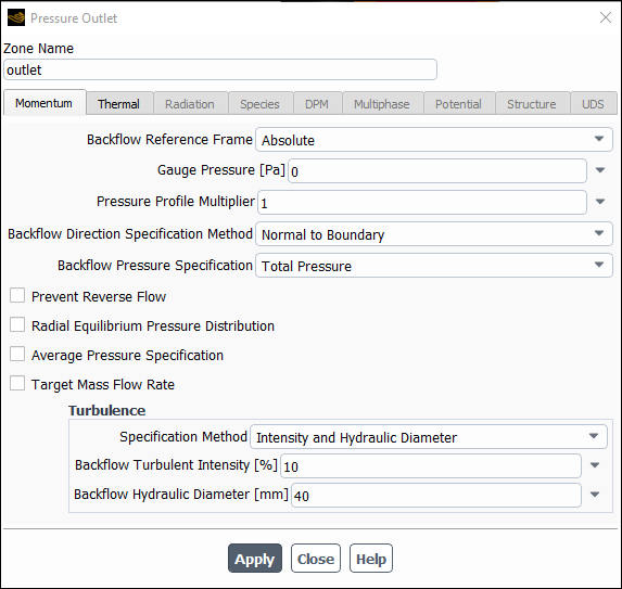
1. Retain the default setting of 0 for Gauge Pressure.
2. In the Turbulence group box, select Intensity and Hydraulic Diameter from the Specification Method drop-down list.
3. Enter a value of 10% for the Backflow Turbulent Intensity.
4. Enter 40 mm for the Backflow Hydraulic Diameter.
5. Click Apply and close the Pressure Outlet dialog box.
Set the wall heat transfer boundary conditions.
Setup → Boundary Conditions → Wall → solid_up:1 Edit...
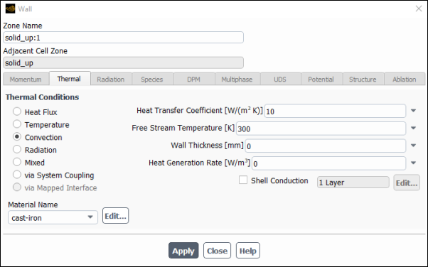
1. Select Convection under Thermal Conditions.
2. Enter 10 for the Heat Transfer Coefficient.
3. Enter 300 for the Free Stream Temperature.
4. Click Apply and close the Wall dialog box.
Apply the same conditions to the other walls (in1, in2, in3, and out1).
1. Select solid_up:1 from the Boundary Conditions node of the Outline View, right-click and select Copy from the context menu.
  This opens the Copy Conditions dialog box.
2. Select in1, in2, in3, and out1 from the To Boundary Zones list.
3. Click Copy, click OK in the confirmation prompt, and close the Copy Conditions dialog box.
Retain the remaining default (wall and interior) boundary conditions.

1.4.10. Solution

Specify the discretization schemes.
In the Solution ribbon tab, click Methods... (Solution group box).
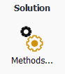Solution → Solution → Methods...

Retain the default settings.
Create a surface report definition of the velocity at the outlet (outlet).
Solution → Reports → Definitions → New → Surface Report → Facet Maximum...

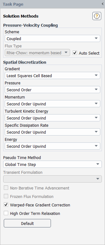
Note: You can also access the Surface Report Definition dialog box by right-clicking Report Definitions in the tree (under Solution) and selecting New/Surface Report/Facet Maximum... from the menu that opens.
1. Enter point-vel for the Name of the report definition.
2. Enable Report File, Report Plot, and Print to Console in the Create group box.
  During a solution run, Ansys Fluent will write solution convergence data in a report file, plot the solution convergence history in a graphics window, and print the value of the report definition to the console.
3. Select Velocity... and Velocity Magnitude from the Field Variable drop-down lists.
4. Select outlet from the Surfaces selection list.
5. Click OK to save the surface report definition and close the Surface Report Definition dialog box.
  The new surface report definition point-vel will appear under the Solution/Report Definitions tree item. Ansys Fluent also automatically creates the following items:
  - point-vel-rfile (under the Solution/Monitors/Report Files tree branch)
  - point-vel-rplot (under the Solution/Monitors/Report Plots tree branch)
Monitor the mass flow rate at the inlets.
Solution → Reports → Definitions → New → Flux Report → Mass Flow Rate...
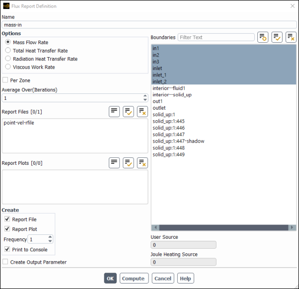
1. Enter mass-in for the Name of the report definition.
2. Select Mass Flow Rate under Options.
3. Select in1, in2, in3, as well as inlet, inlet_1, inlet_2 from the Boundaries selection list.
4. Enable Report File, Report Plot, and Print to Console in the Create group box.
5. Click OK to save the surface report definition and close the Flux Report Definition dialog box.
  The new surface report definition mass-in will appear under the Solution/Report Definitions tree item. Ansys Fluent also automatically creates the following items:
  - mass-in-rfile (under the Solution/Monitors/Report Files tree branch)
  - mass-in-rplot (under the Solution/Monitors/Report Plots tree branch)
Monitor the total mass flow rate through the entire domain.
Perform the same procedure as described above, naming the report mass-tot, and selecting all boundaries.
Monitor the mass balance.
Use expressions to create a report definition for the mass balance using existing report definitions.
Solution → Reports → Definitions → New → Expression...
This opens the Expression Report Definition dialog box.
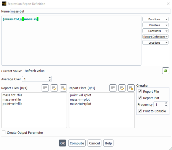
1. Enter mass-bal for the Name of the expression.
2. Select mass-tot from the Report Definitions drop-down list on the right.
3. Type the / operand.
4. Select mass-in from the Report Definitions drop-down list on the right.
5. Enable Report File, Report Plot, and Print to Console in the Create group box.
6. Click OK to save the expression definition.
Initialize the flow field using the Initialization group box of the Solution ribbon tab.
Solution → Initialization
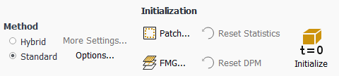
1. Select Standard from the Method list.
2. Click Initialize.
Save the case file (manifold_solution.cas.h5).
File → Write → Case...
Start the calculation by adjusting the time scale factor to 5 and requesting 100 iterations in the Solution ribbon tab (Run Calculation group box).
Solution → Run Calculation
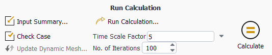
1. Change the Time Scale Factor to 5.
2. Enter 100 for No. of Iterations.
3. Click Calculate to begin the iterations.
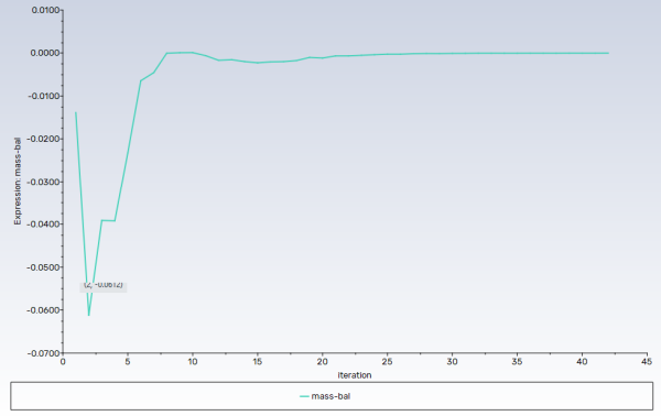
  As the solution progresses, the mass flow rate graph flattens out, as seen in Figure 1.2: Mass Flow Rate History.
  Figure 1.2: Mass Flow Rate History
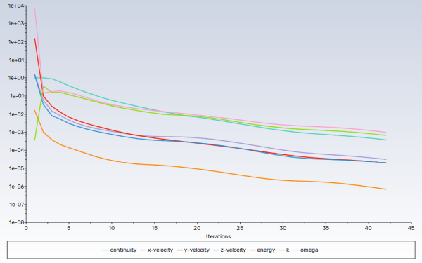
4. Similarly, the residuals history will be plotted in the Scaled Residuals tab in the graphics window (Figure 1.3: Residuals).
  Figure 1.3: Residuals
Save the case and data files (manifold_solution.cas.h5 and manifold_solution.dat.h5).
File → Write → Case & Data...

1.5. Postprocessing

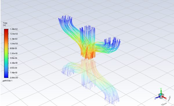
Display path lines highlighting the flow field (Figure 1.4: Pathlines Through the Manifold).
Results → Graphics → Pathlines → New...
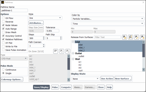
1. Keep the default of pathlines-1 for the Name.
2. Select Particle Variables... and Time from the Color by drop-down lists.
3. Set the Path Skip value to 5.
4. Select Accuracy Control from the Options list.
5. Select inlet, inlet_1, and inlet_2 from the Release from Surfaces list.
6. Click Save/Display and close the Pathlines dialog box.
  The new pathlines-1 definition appears under the Results/Graphics/Pathlines tree branch. To edit your surface definition, right-click it and select Edit... from the menu that opens.
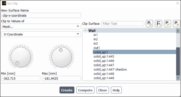
  Figure 1.4: Pathlines Through the Manifold
Create two clipped surfaces through the manifold geometry.
Results → Surface → Create → Iso-Clip...
1. Create Surface 1
  1. Enter clip-x-coordinate for Name.
  2. Select Mesh... and X-Coordinate from the Clip to Values of drop-down lists.
  3. Select solid_up:1 from the Clip Surface list.
  4. Click Compute.
  5. Keep the Min value at its minimum setting, and adjust the Max value to be at its halfway point.
  6. Click Create.
    The new clip-x-coordinate definition appears under the Results/Surfaces tree branch. To edit your surface definition, right-click it and select Edit... from the menu that opens.
2. Create Surface 2
  1. Enter clip-z-coordinate for Name.
  2. Select Mesh... and Z-Coordinate from the Clip to Values of drop-down lists.
  3. Select solid_up:1 from the Clip Surface list.
  4. Click Compute.
  5. Keep the Min value at its minimum setting, and adjust the Max value to be at -44.0 .
  6. Click Create and close the Iso-Clip dialog box.
    The new clip-z-coordinate definition appears under the Results/Surfaces tree branch. To edit your surface definition, right-click it and select Edit... from the menu that opens.
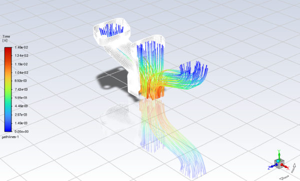
Create a scene containing the mesh and the path lines.
Results → Scene New...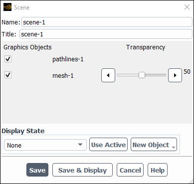
1. Keep the default scene-1 for the Name.
2. Enable the pathlines-1 graphics object.
3. Create a new mesh object to add to the scene.
  1. Click New Object and select Mesh to open the Mesh Display dialog box.
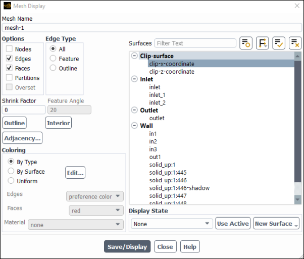
  2. Ensure that Edges is selected under the Options list.
  3. Select clip-x-coordinate under the Surfaces list.
  4. Click Save/Display and close the Mesh Display dialog box.
    The new mesh-1 definition appears under the Results/Graphics/Mesh tree branch. The new object also appears in the Scene dialog box.
4. In the Scene dialog box, set the Transparency of mesh-1 to 50.
5. Click Save & Display and close the Scene dialog box.
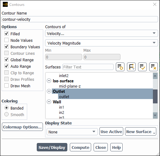
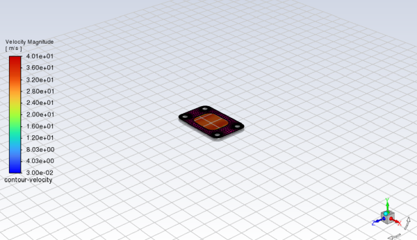
  Figure 1.5: Scene Containing the Mesh and Pathlines Throughout the Manifold
Create and define contours of velocity magnitude at the outlet along with the mesh.
Results → Graphics → Contours → New...
1. Enter contour-velocity for the Name.
2. Select Velocity... and Velocity Magnitude from the Contours of drop-down lists.
3. Select outlet from the Surfaces list.
4. Disable Node Values under Options.
5. Enable Draw Mesh under Options.
  This displays the Mesh Display dialog box.
  
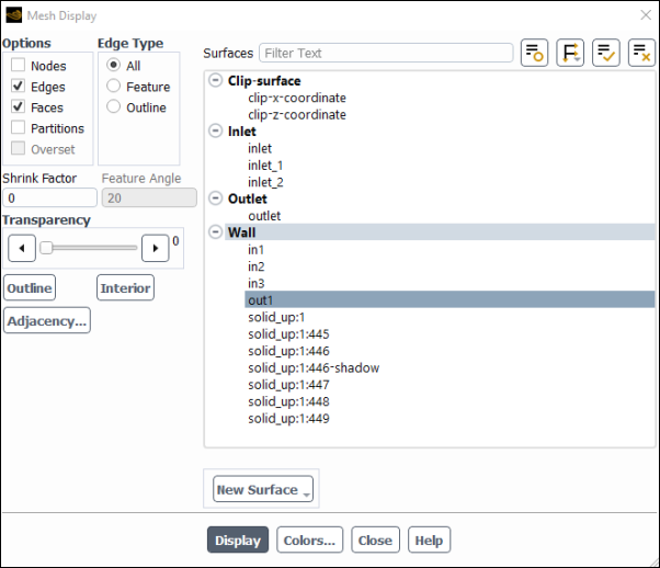
  In the Mesh Display dialog box, deselect all surfaces, select the out1 surface, click Display and close the dialog.
6. Click Save/Display and close the Contours dialog box.
Figure 1.6: Contours of Velocity Magnitude at the Outlet
Create an iso-surface through the manifold geometry.
Results → Surface → Create → Iso-Surface...
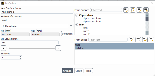
1. Enter mid-plane-z for Name.
2. Select Mesh... and Z-Coordinate from the Surface of Constant drop-down lists.
3. Select fluid1 and solid_up from the From Zones... list.
4. Click Compute.
  The Min and Max fields display the Z extents of the domain.
5. Enter -44 for the Iso-Values.
6. Click Create and close the Iso-Surface dialog box.
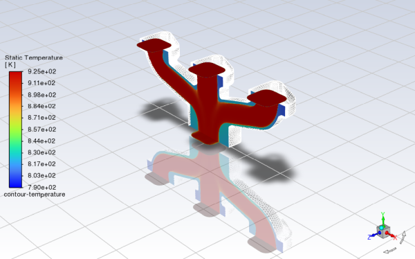
Create and define a contour of temperature along the mid-plane.
Results → Graphics → Contours → New...
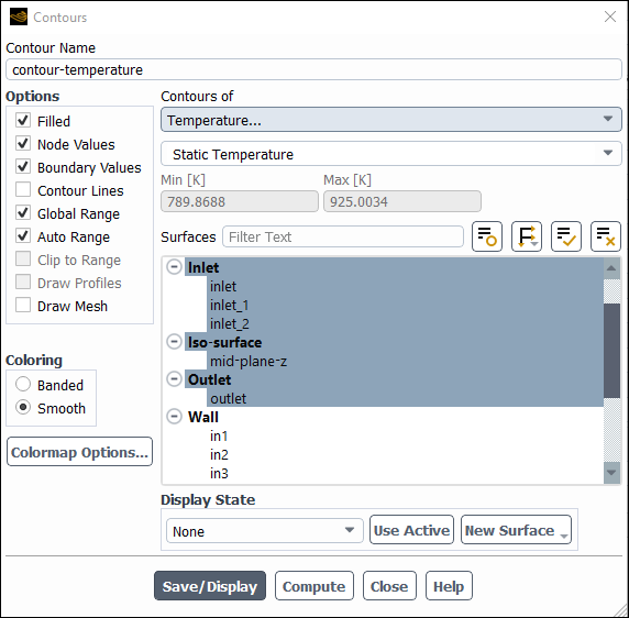
1. Enter contour-temperature for the Name.
2. Select Temperature... and Static Temperature from the Contours of drop-down lists.
3. Select inlet, inlet_1, inlet_2, mid-plane-z, outlet, and out1 from the Surfaces list.
4. Enable Draw Mesh under Options.
  
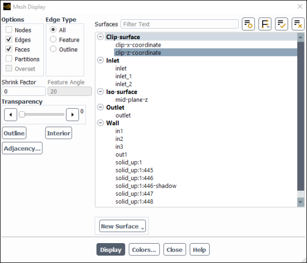
  In the Mesh Display dialog box, deselect all surfaces, select the clip-z-coordinate surface, click Display and close the dialog.
5. Click Save/Display and close the Contours dialog box.
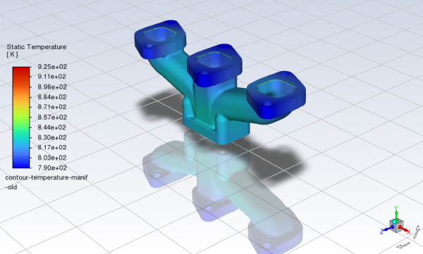
Figure 1.7: Contours of Temperature at the mid-plane
Create and define a contour of temperature for the manifold geometry.
Results → Graphics → Contours → New...
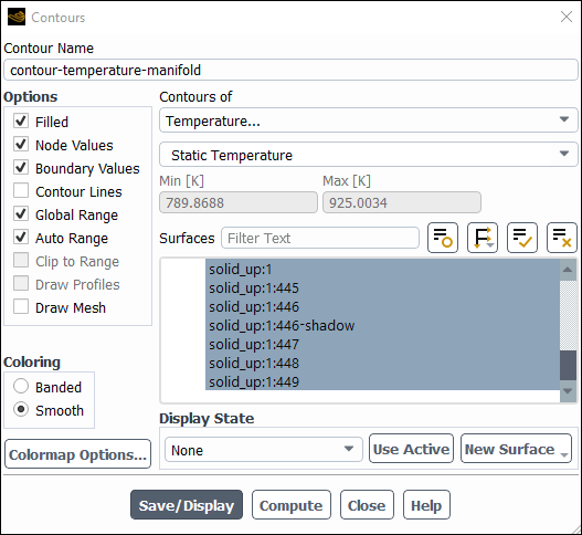
1. Enter contour-temperature-manifold for the Name.
2. Select Temperature... and Static Temperature from the Contours of drop-down lists.
3. Select the Wall group from the Surfaces list.
  Click to deselect all surfaces. Click and select Surface Type under Group By to list the surfaces by type, as shown above.
4. Click Save/Display and close the Contours dialog box.
Figure 1.8: Contours of Temperature on the Exhaust Manifold
Save the case and data files (manifold_solution.cas.h5 and manifold_solution.dat.h5).
File → Write → Case & Data...
You will use these case and data files in Fluent Postprocessing : Exhaust Manifold.

1.6. Summary

In this tutorial, you learned how to import a CAD geometry, generate a volume mesh, and set up, solve, and postprocess a CFD problem involving air flow and heat transfer through a manifold all within a single Ansys Fluent interface.

Related video that demonstrates steps for setting up, solving, and postprocessing the solution results for a turbulent flow within a manifold: