


Once the grid and input parameters have been defined, click the Run
icon ![]() to launch the calculation.
to launch the calculation.
A new window opens to control and monitor the calculation. If you are already in the
FENSAP-ICE Solver Manager window, click the button  at the bottom of the window to switch to the
Run environment. You can always return to the input parameter
environment by clicking the button at the bottom of the
window.
at the bottom of the window to switch to the
Run environment. You can always return to the input parameter
environment by clicking the button at the bottom of the
window.
The input parameters cannot be modified after the execution has started.
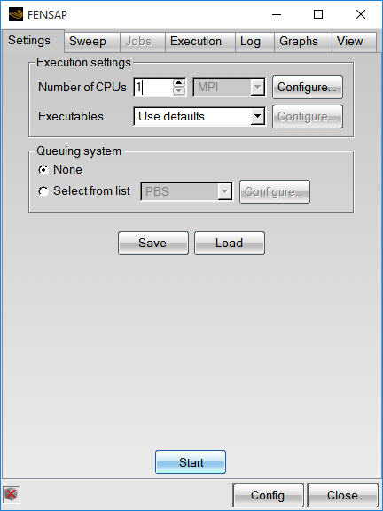
The run configuration window shows the configurable execution settings:
FENSAP, DROP3D, ICE3D, OptiGrid all use the Open MPI (Message Passing Interface) library to significantly shorten the solution time for large-scale problems. The grid is first partitioned with ParMETIS (courtesy of George Karypis, Kirk Schloegel and Vipin Kumar, copyright University of Minnesota). Then each processor operates on its own (smaller) subdomain grid and exchanges information with the other processors through the Open MPI interface.
Enter the Number of CPUs to be used by the solver.
The mpirun command is used by default to launch the MPI
solvers. On some machines, however, this command must be customized. To do so,
click the button. A new window opens to
prompt for the MPI command line:
If necessary, override the standard mpirun command and
browse to select the appropriate mpirun wrapper to be used by MPI.
If necessary, add the appropriate optional parameters required by the mpirun wrapper to manage the parallel calculation.
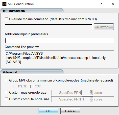
The resulting complete command line is displayed for verification before the execution is started.
Additional custom settings can be defined in the Advanced
section. Group MPI jobs on a minimum of compute-nodes is
useful for CHT3D computations where the flow solver executes on more
processors and for longer times before inter-processor synchronization than
either ICE3D or C3D. This option allows ICE3D and C3D to run
compactly and more efficiently on fewer cores than the flow solver, without
being broken-up across all the nodes. A custom machinefile
is required to enable this option. The custom machinefile
is assigned in the Additional mpirun parameters box by
specifying the MPI option -machinefile machinefile_name.
The custom machine file should list the cores of each node in sequential
order.
Note: Refer to MPI for additional information and troubleshooting help concerning the configuration of MPI on clusters and multi-core machines.
The last two options, Custom compute-node size and Custom master-node size are only active for OptiGrid. If either of the two values is set to a value smaller than the number of cores per node, fewer cores per node will be used and more memory is available to the active cores.
The application can be launched using different queuing systems (PBS, SGE, MOAB, AT, GUI, NULL, CUSTOM). If no queuing system is installed on the machine, select None.
Additional parameters can be added for each queuing system by clicking the button. These parameters are specific to each queuing system. See MPI for more information.
Calculations are launched by clicking the Start button. Once the calculation is launched, the background color of the run in the main window will change.
FENSAP can automate the computation of the drag polar curves by launching a sequence of computations with different angles of attack (or yaw angle). To do so, enter the minimum and maximum angles of attack (or yaw angles), as well as the number of increments, in the appropriate Sweep variable boxes. The step is automatically displayed.
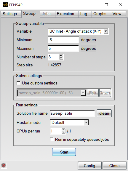
To speed-up the solution process, set the total number of CPUs and distribute them equally for each calculation. In the example shown above, 8 FENSAP runs will be computed using 4 CPUs each. Since only 16 CPUs have been assigned in Settings, FENSAP-ICE will run 2 sequential sets of 4 concurrent angles of attack (or runs).
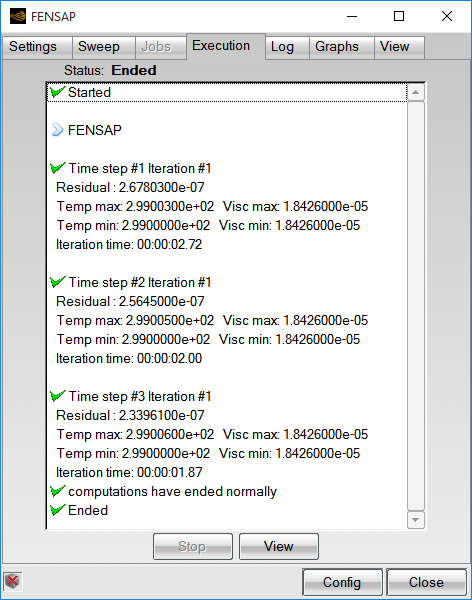
The main solver execution steps can be monitored: read grid, read initial solution, compute each time step, etc. Successful completion or error messages, if any, are displayed in the window.
The log section shows the output file of the solver. Its contents vary from solver to solver. The output file should be kept in the run directory since it can be essential in obtaining quick technical support from Ansys.
The graph mode monitors the convergence graphs. Different variables can be plotted depending on the solver. For example:
Residuals of the momentum, energy and turbulence equations (FENSAP)
Residuals of the continuity and momentum equations (DROP3D)
Lift and drag coefficients (FENSAP)
Classical and Gresho total heat (FENSAP)
Total collection efficiency (DROP3D)
Convergence of the GMRES linear matrix solver (FENSAP, DROP3D)
Probe point values (FENSAP, DROP3D)
Mass and energy conservation (FENSAP)
Total mass of accreted ice (ICE3D)
Time variation of the film height, temperature and, rate of ice accretion (ICE3D)
Minimum and maximum temperatures (C3D, CHT3D)
Number of nodes and elements (OptiGrid)
Error distributions before and after mesh adaptation (OptiGrid)
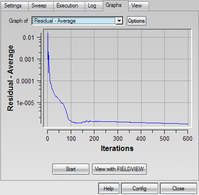
The axis of the graph can be changed and the convergence curve saved and printed by clicking the Options button.
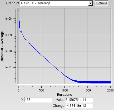
Click the convergence window to display the exact value at the cursor location (vertical red line). Dragging while holding the left mouse button allows the cursor to move along the curve. The X- and Y-axis values are shown below the graph. Clicking the right mouse button cancels the graph probe.
Hold Shift and drag horizontally to zoom along the X-axis. Hold Shift and drag vertically to zoom along the Y-axis. The zoom region is then highlighted in yellow until the mouse button is released.
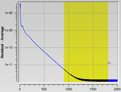
Hold Shift and click the left mouse button in the convergence window to zoom out, or click the middle mouse button.