


In this section you will set up various conjugate heat transfer options using CHT3D.
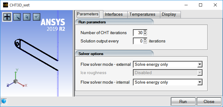
The number of CHT3D iterations, for example, the number of loops through all the domains to exchange information can be set in the Run parameters section. The solutions of all the domains can be saved every few iterations if desired.
When FENSAP is the flow solver, the Flow solver mode box under Solver options offers the choice of four solution modes: (default), , or In the case of Fluent and CFX, the Flow solver mode box only offers these options: Solve full Navier-Stokes and Use heat transfer coef..
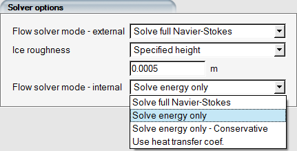
In the mode, the continuity and momentum equations of the fluid in each domain are frozen, only the energy equation is solved. The mode allows a full viscous solution in each fluid domain, however this mode can be computationally expensive. The option solves the conservative energy equation which is recommended if the free stream Mach number is in the transonic range. Finally, the option simplifies the problem by modeling the heat exchange with the fluid domains using the convective heat transfer coefficient and a reference temperature. While the reference temperatures are taken from the parameters of each fluid run, the heat transfer coefficient is automatically computed using the initial solution temperature and heat flux distribution.
When the external flow solver mode is set to , the Ice roughness height option can be enabled. This option improves the ice shapes computed by CHT3D by imposing roughness where ice forms. The shear stress and heat flux of the ice patches will change accordingly, while uncontaminated regions will remain smooth. Two roughness options are available:
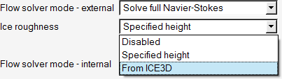
The Specified height option uses a constant value of sand grain roughness for the iced surfaces in the anti-icing simulation. option inherits the ice roughness calculated by ICE3D using one of its roughness models (beading, NASA roughness, Shin & Bond, etc.)
Note: Fluent and CFX will automatically apply this roughness using the High roughness (Icing) model. The Roughness Constant is always set to 0.5. It will also enable the Blended Near Wall treatment of CFX.
If the initial Fluent solution was computed using serial or parallel solver execution, the same parallelization setting should be used in the subsequent CHT execution. Fluent might reorder the nodes of the grid when switching between serial and parallel execution, making the reordered grid unsuitable for FENSAP-ICE restarts. You should always use the parallel version of Fluent, to avoid mismatched files. In the case of CFX, only parallel runs are supported. Therefore, two or more cores should be specified.
Values for the time-step and convergence loops are set in the Parameters panel of the CHT de-icing configuration.
Similar to the standalone C3D module, two time stepping schemes are provided in de-icing CHT: Constant and Automatic modes. The Constant mode employs a constant time step throughout the simulation, while with the Automatic option, the time step is determined by the rate of heat conduction and the element size. The Maximum time step sets the maximum upper limit of the auto-computed time step.
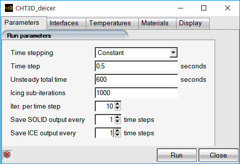
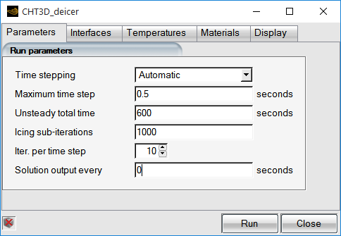
The Unsteady time step parameter sets the global time step of the CHT loop. The Unsteady total time is the total time of the CHT simulation.
Within each CHT time step, the water film, ice and solid domains will be solved sequentially and repeatedly until thermodynamic balance is reached at the interfaces. The number of times each domain is solved is controlled with Iter. per time step parameter.
Note: Select a number of Iter. per time step large enough to
converge the solid minimum and maximum temperature at each time step. The solid
temperature convergence graphs are displayed at runtime in the
Graph tab of the run window. By default, the value is
set to 10 which is very conservative. You can reduce this value to
3 to speed-up calculations, if min/max solid
temperature per time step is stable by then.
At each time step, the solution of each domain advances for a total duration corresponding to the Unsteady time step. While the solid and phase-change solvers can march with the same time step as the CHT loop, the water film solution requires much smaller time steps for stability. Hence, each CHT Unsteady time step is divided into a given number of smaller intervals to compute the water film solution. The number of time steps of the film domain is defined with the Icing sub-iterations parameter. For example, using an Unsteady time step of 0.1 s and 1000 Icing sub-iterations, the film solution will be computed at each CHT time step using 1000 inner time steps of 1E-04 s, while the conduction and phase change through the solid and ice layer domains will advance using a single time step of 0.1 s. You should consider using in ICE3D to potentially use a larger local time step and reduce the cost of icing calculations.
The Conjugate Heat Transfer procedure requires the application of a specific solver in each domain, hence the domain interfaces must be configured in order to apply the appropriate interface conditions.
Go to the Interfaces panel to configure the interfaces between the fluid and solid domains.
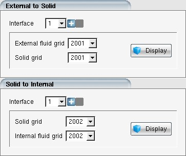
Each interface is defined in terms of a pair of wall boundary condition indices that connect a fluid domain to one side of the solid domain. Select the boundary condition indices of the fluid and the solid domain that correspond to the common interface.
Multiple interfaces are supported. To add an interface, click the  button and pair the wall families that form the interface. To
delete an interface, click the
button and pair the wall families that form the interface. To
delete an interface, click the  button.
Click the buttons to visually verify the correctness of the coupling of each pair of wall families in the graphical window.
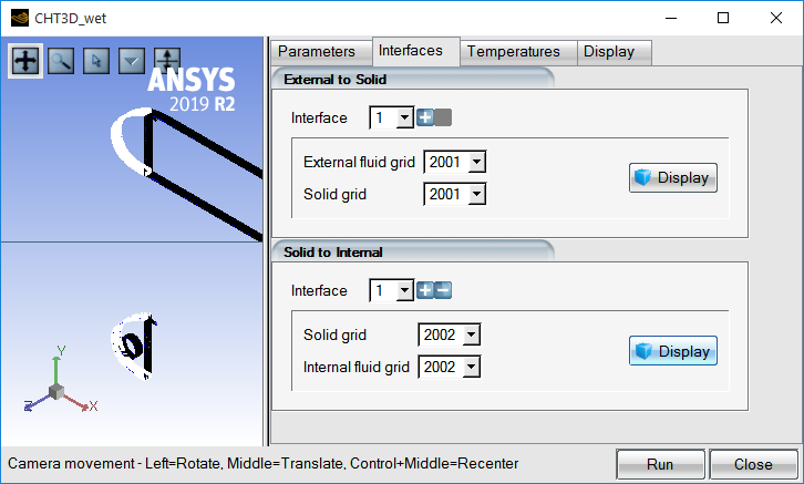
Note: Only wall boundary condition indices are shown by the graphical interface.
CHT3D takes care of the information exchange through the interfaces automatically, even if the two surfaces don’t match point-by point.
To obtain accurate CHT solutions, especially in the wet air regime, it is imperative that the CHT3D reference temperatures be set correctly. CHT3D uses two reference temperatures to compute convective heat transfer coefficients from the heat fluxes, the External surface recovery temperature and the Internal adiabatic stagnation temperature. The two temperatures are detected automatically by FENSAP-ICE when FENSAP is the main flow solver, hence these parameters are not editable.
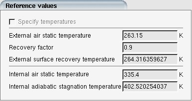
Other flow solvers, such as Fluent or CFX, may not provide this critical data automatically, therefore when the flow solver is other than FENSAP, the Specify temperatures check box is activated automatically and the correct reference temperature values must be initialized manually. Refer to The Recovery Factor for more details on how to compute the External surface recovery temperature.