


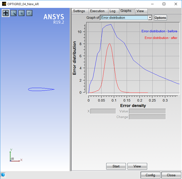
Click Run to start the adaptation. Refer to The FENSAP-ICE Solver Manager for guidelines on how to use both the Execution and Graphs windows.
OptiGrid shows at conclusion of mesh adaptation the initial and adapted grids in the graphical window. You can change the boundaries displayed by OptiGrid under the Boundaries menu.
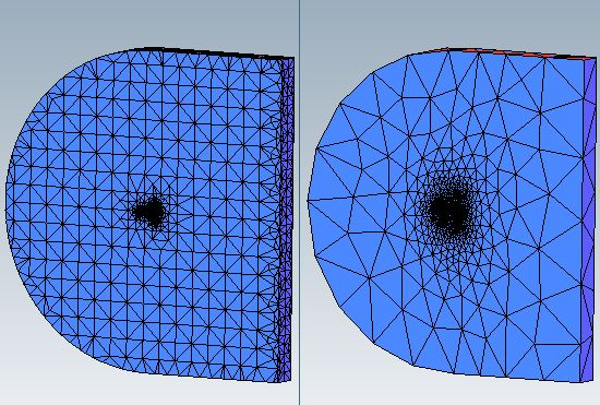
Click the side-by-side icon  to display the initial grid on
the left and the adapted grid on the right.
to display the initial grid on
the left and the adapted grid on the right.
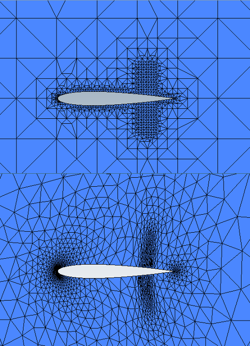
Click the up-and-down icon  to display the initial grid in the upper section of the window, and the adapted
grid in the lower section.
to display the initial grid in the upper section of the window, and the adapted
grid in the lower section.
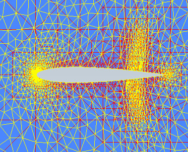
Finally, click the last icon  to overlay the initial and adapted
grids.
to overlay the initial and adapted
grids.
If Viewmerical is your default post-processing tool defined in the preferences, use the button in the run panel. Viewmerical will permit to display the grid boundaries and also cutting planes onto the volume. Refer to Post-Processing.
Viewmerical can display all grid types supported by OptiGrid.
OptiGrid is closely linked to the flow solver. Generally, several loops between the flow solver and OptiGrid should be performed in order to obtain a final adapted grid with an accurate flow solution. The process can be summarized as follows:
Given a mesh Mn at loop n, compute the solution Sn on this mesh with the flow solver;
OptiGrid estimates the error of Sn over all edges of Mn;
OptiGrid produces a new mesh Mn+1 using edge refinement, coarsening, swapping and node movement, and interpolates the solution Sn+1/2 from Sn on Mn+1;
A solution Sn+1 on Mn+1 is then computed by the flow solver, starting with the interpolated solution Sn+1/2 provided by OptiGrid as an initial guess;
The loop is repeated until convergence is achieved.
Note: The ability of the flow solver to accept increasingly stretched grids determines how close one gets to an optimum grid. Most well-written unstructured flow solvers are capable of accepting grids that are increasingly, but gradually, stretched.
The following tips are designed to help you run OptiGrid in the most effective way possible.
Make sure your CAD data is properly and completely defined.
The most common source of problems when using OptiGrid is poorly defined CAD data. OptiGrid is quite sensitive to messy CAD data and problems will often become apparent only after OptiGrid has been used to adapt the mesh. If these problems appear, it will be necessary to go back to the CAD geometry and repair the troublesome areas of the geometry. For example, make sure curves are well-defined at the junction of non-tangential surfaces.
It is better to start with a dense mesh rather than with a mesh that is too coarse.
It is a good idea to start with an initial mesh that has a higher density rather than a lower one, for several reasons. To start with, the geometry may not be properly represented by an initial mesh that is too coarse, especially if it is complex or has highly curved surfaces. Since the CAD is reconstructed from the initial mesh, it is important to have a high-resolution mesh on rounded surfaces for quality adaptation. OptiGrid is also more likely to have trouble refining the mesh on high curvature areas if the mesh is too coarse. It is much easier to coarsen on curved surfaces than to refine. Also, if the initial mesh is too coarse, the solution is less likely to capture the important characteristics of the flow and the adaptation may make the mesh worse rather than better.
Run OptiGrid in the smoothing mode (without a solution) before starting the solution, to ensure that there are no elements with a very small aspect ratio.
Examine the flow solution before starting the adaptation.
Make sure the solution is sufficiently converged before starting the adaptation to ensure that the dominant flow characteristics are captured.
Use the target number of elements or target number of nodes option.
The easiest way to run OptiGrid is to select the or . With these options, you can set the final size of the adapted mesh and OptiGrid will approximate the target error density so as to match that size. The main iterations should be between 5 and 15.
Set the mesh constraints based on the current mesh. Verify the minimum and maximum edge lengths.
Gradually increase the total number of nodes/elements, do not abruptly increase the mesh size.
Do not expect to adapt in one solver-adaptation cycle (3 or more cycles are generally required).