


The unsteady solution process consists of one or more cycles, during which heating elements may be turned on or off through changes of the boundary conditions.
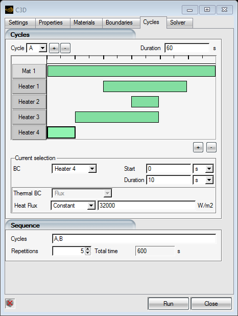
To add or remove boundary condition cycles, click or . All boundary condition cycles are shown graphically and sequentially in the cycle bar at the top. To select one cycle, click the bar corresponding to that cycle. The bar will then be highlighted in blue.
Each cycle starts at the end of the previous cycle. Set the cycle duration in the Duration box, in seconds. The total time is then shown as the sum of all cycles.
For each cycle, set the heating element boundary conditions to be imposed. Heaters can be turned on by clicking the On button and by imposing the corresponding heat flux. Specify the power density for (Mat). The other boundary conditions can be left as default or modified in this menu.
A Cycle defines the state of boundary conditions, heater pads or volumetric heat sources for a given period of time. To add or remove cycles, click or button on the top left of the Cycle graph. Cycles are identified with letters and can be selected in the Cycle drop box. Set the cycle duration, in seconds, in the top right Duration box. Boundary conditions for walls, heater pads, and volumetric heat sources can be added in or removed from each cycle by clicking the or button on the bottom right of the Cycle graph. All boundary condition cycles are shown graphically.
To modify a defined boundary condition within the current cycle, click the green bar corresponding to that object to enable editing. The bar will then be highlighted. The Start and Duration can be toggled between seconds (s) and percentage (%). If the cycle is resized, boundary conditions set-up in % will be rescaled to the new cycle length. The default duration type is in percentage (%) of the cycle duration.
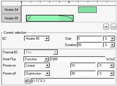
The heating pad Heat Flux can be set either to Constant or Function. In Constant mode, the heat flux change is instantaneous. In Function mode, Power-on and Power-off transitions can be configured. Various functions can be supplied:
Linear: The power increases from the default state to the defined power value in a linear fashion from activation for a specified duration (in seconds or %).
Expression: The power changes according to the given expression. The expression uses the relative time (T) variable, which is automatically set by FENSAP-ICE to 0 at the start of the power-on period and 1 at the end. You must ensure that the expression f(T) returns 0 at the start and 1 at the end and that 0 ≤ f(T) ≤ 1 over the interval 0 ≤ T ≤ 1.
Power-on functions for a 10-second activation period:
Linear: T
Power law: T^0.3
The syntax of the expression language is described in Expression Syntax.
Note: For Power-down, the expected values are reversed. The expression should return 1 at the start of the power-off period and 0 at the end.
Power-down functions for a 5-second deactivation period:
Linear: 1-T
Power law: (1-T)^0.3
A Sequence is a combination of one or multiple Cycles. Any sequence of cycles can be entered, with the cycle name identifiers separated by a comma (such as A if there is a single cycle, or A,B or A,B,A,C,C for more complex sequences). Each cycle starts at the end of the previous cycle. The global repetition of sequences can be performed by providing the repetition number. Modify the repetition number directly or click the up and down arrows to change it. The total time will be automatically computed and then shown as the sum of all cycles.