


Several options are available to customize FENSAP's output to suit your particular needs.
The output log level is configurable in the Out page.
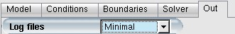
Table 4.3: Pull Down Menu Options
| Minimal | Reduces log size to a minimum, less printout at each iteration. |
| Default | Regular log output. |
| Detailed | Includes extra information, such as timing for each subroutine. |
The FENSAP solution is saved in FENSAP format (See FENSAP-ICE File Formats for format details).
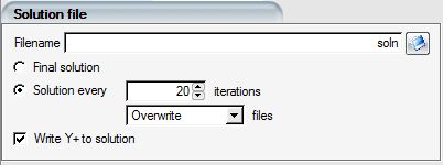
The solution can be saved either at the end of the calculation (Final solution) or at fixed intervals during the iterative solution process. When saving the output file every N iterations, the solution can be either overwritten (Overwrite) or saved in separate files numbered with the iteration/time step number (Do not overwrite).
Tip: If turbulence is enabled, computing the y+ and u+ data on large grids could be costly. If these variables are not important, their computation can be disabled by clearing the box: Write Y+ to solution.
When solving for unsteady flows, the solution can be saved at fixed intervals in time to enable animations.
For moving boundaries, for example, mesh displacement due to ice accreting in time or body motion, FENSAP uses the ALE (Arbitrary Lagrangian Eulerian) formulation.
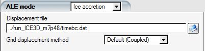
There are two displacement methods, coupled and uncoupled. The coupled method solves for the displacements in the x-, y-, and z-direction simultaneously, providing a better distribution of the effect of surface displacement into the interior of the computational domain. This approach yields good mesh orthogonality and element quality near the surface, however it is somewhat more computationally expensive than the uncoupled solution. The default Coupled option is therefore recommended.
Mesh movement can be performed in two cases:
In the case of multishot ice accretion, the surface displacement due to ice accretion is obtained as an output from ICE3D. The timebc.dat file from ICE3D should be assigned to FENSAP using the Browse button. In this quasi-steady mode, the displacement velocity is not included in the flow solution.
With aero-elasticity (unsteady flows with moving boundaries), the displacement velocity is computed at each time step and the mesh is automatically displaced by FENSAP. In this unsteady mode, the displacement velocity is included in the flow solution.
Important: The 6000 and 7000 boundary condition families, which are actuator disks, screens, heater pads, and interfaces are not allowed to deform due to mesh displacement from icing. Therefore it is important to make sure these boundaries are not in contact with ice accreting walls to begin with.
FENSAP computes the resultant force F acting on all solid surfaces of the grid. This force can be split into lift and drag. If your grid contains symmetry planes that touch wall boundaries, the force components in the symmetry directions will be removed from this resultant force before splitting it into lift and drag components.
Note: The lift calculation is not accurate for periodic grids.
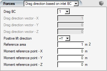
The positive lift direction represents the up direction which will help determine the sign of the final reported lift. The lift coefficient is computed as follows:

where the lift  is equal to resultant force along the lift direction, and
 is the reference area.
The drag vector  is the projection of the resultant force
  along the drag direction. The drag coefficient is computed as
follows:
along the drag direction. The drag coefficient is computed as
follows:

The moment is the summation over all wall faces of the local force times the normal distance between its point of action and the
moment center specified in Moment reference point -X, -Y and
-Z.
Important: FENSAP writes extensive information on the lift and the drag and their coefficients. The intermediate and final values appear in the log file, along with their breakdown by surface index. Intermediate values of the lift and drag coefficients are also displayed in the convergence graphs. You should pay special attention to these two quantities to ensure proper convergence of the flow solver.
: The drag direction is set in the same direction as the velocity of the inlet boundary selected in the Drag BC window.
: The non-dimensional direction components are provided by you in the Drag direction vector -X, -Y and -Z boxes.
: The lift and drag are not computed by FENSAP.
Note: The sign of the lift coefficient depends on the orientation of the body. You should specify the approximate positive lift direction.
Click the blue icon ![]() to display the drag vector in the graphical window. Click again
to remove the display.
to display the drag vector in the graphical window. Click again
to remove the display.
Probe points can be defined in the computational domain to monitor the flow solution at specific locations during convergence.
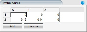
To do so, click the button and enter the (X,Y,Z) coordinates of each probe point.
Click the blue icon ![]() to view the probes in the graphical window. Click again to
remove the probes from the graphical view.
to view the probes in the graphical window. Click again to
remove the probes from the graphical view.