


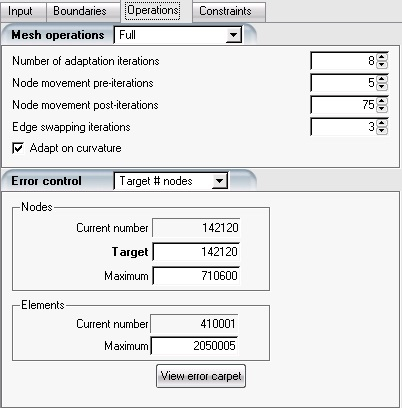
OptiGrid gives the choice of adapting the grid using:
mesh optimization including adding/removing nodes, edge swapping and node movement. This strategy is strongly recommended as the combination of all adaptive strategies allows equidistributing the error throughout the computational domain more effectively.
combines only adding/removing nodes with node movement.
should only be used with hexahedral grids where nodes cannot be added nor deleted.
Number of adaptation iterations sets the number of cycle performed by OptiGrid, starting from the initial grid and flow solution, to the adapted mesh and the flow solution interpolated onto that new grid.
Note: If the initial grid is well suited to the flow, the mesh adaptation may not require more than 3 main iterations. On the other hand, if the initial grid is uniform or very coarse, the mesh adaptation process may require up to 15 main iterations.
Node movement pre-iterations sets the maximum number of node movement loops in stages 1 and 3 of the adaptation sequence.
Node movement post-iterations sets the maximum number of node movement loops at stage 6 of the adaptation sequence.
Edge swapping iterations sets the maximum number of edge swapping loops at stage 5 of the adaptation sequence.
Adapt on curvature is enabled by default, and controls the activation of curvature-only refinement & swapping operations. With this option enabled, OptiGrid might refine edges on surfaces where the maximum coarsening on curvature setting suggests it, even if the adaptation metric does not imply refinement at this location.
If this option is disabled, OptiGrid will still constrain all operations to be compliant to the curvature defined by the CAD. This option can be useful to avoid curvature-only refinement on a curved surface (such as a far-field) with a low error solution.
Adaptation on curvature was always enabled in previous versions of OptiGrid.
OptiGrid gives you several options for setting the error density:
In Automatic mode, OptiGrid auto-selects the error density based on the current number of elements in the initial grid. This option is useful to obtain a first estimate of the error density.
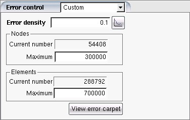
In Custom mode, OptiGrid equidistributes the error to match the specified Error density. Click
 to display the error density.
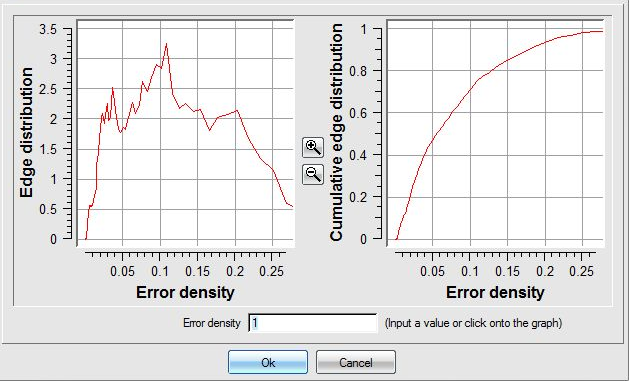
The graph (left) presents the error computed on the initial grid as a function of the percentage of the total number of edges. A good initial guess for the target error density can be obtained by viewing the cumulative error distribution (right) and selecting the error that corresponds to the 70th percentile of the distribution.
With , OptiGrid auto-selects and adjusts the error density so as to obtain a specified target number of elements set under Target/Elements. Note that it is acceptable, within OptiGrid, to momentarily exceed the specified target number of elements.
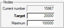
With , OptiGrid auto-selects and adjusts the error density so as to obtain a specified target number of nodes set under Target/Nodes.
Note: It is acceptable, within OptiGrid, to momentarily exceed the specified target number of nodes.
For options target # elements and target #
nodes, the number of main iterations should be set to
approximately 10, in order to allow a good estimation of
the error density and reach the desired target number of elements or
nodes.
Tip: When performing mesh smoothing, set the error density to
1 to preserve mesh density of the original mesh (with
the Custom option). Reduce this value to refine or increase
it to coarsen.
Maximum in the Nodes group sets the maximum allowable number of nodes. No matter which method of error control is selected, if this limit is reached during the adaptation, OptiGrid will stop refining the mesh until more nodes are eliminated through the coarsening process.

Maximum in the Elements group sets the maximum allowable number of elements. No matter which method of error control is selected, if this limit is reached, OptiGrid will stop refining the mesh and swapping edges until more elements are freed through the coarsening process.
Important: If either of the Maxima is reached during the adaptation process, it is very likely that some patches of the grid have not been adapted and therefore the final grid is not optimal. In this case it is wise to increase the Maxima to a safe level and adapt the grid again.
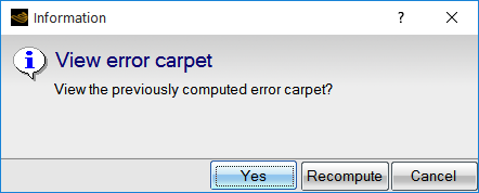
You can compute and view the error carpet (obtained from the input solution) by clicking the button View error carpet. If the carpet is computed already, a message box will appear asking if you want to display the existing error carpet plot or recompute it.
The error carpet is also computed automatically before and after adaptation. It is
then available through the button of the run panel, or
from the error_before.soln/error_after.soln
icons of the project panel.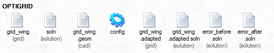
The computation and writing of the error carpet can be switched off (See Error Computation)
In this section you will use OptiGrid's more advanced settings to compute the error carpet.
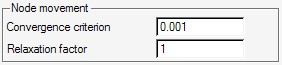
Available only in Advanced solver options mode:
Convergence criterion is the convergence level of the iterative scheme used to solve for node movement. Use a value of 0.001 by default.
The Relaxation factor is the constant in the node movement equation, and should be set to 1 for most applications. It can be reduced to a smaller value if convergence of the iterative process is difficult to achieve. For the adaptation of a hexahedral grid, a value of 0.2 is suggested. Under-relaxation is also recommended when performing Y+ adaptation.
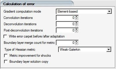
Convolution is used to filter the solution and remove the noise. This operation is achieved by solving a Laplacian equation, which is equivalent to a convolution process with a Gaussian. Convolution iterations is the number of time steps. A value of one is sufficient to remove reasonable numerical oscillations unless the solution is extremely noisy. Adapting on a noisy solution can affect the quality of the adaptation.
When selecting the check box , the error carpet is computed before and after the adaptation, and saved respectively in error_before.soln and error_after.soln. Icons for these files will be added to the list of output files.
The quality of the adapted grid is determined by the quality of the solution. When the original grid is quite coarse, the solution is poor around shocks and across boundary layers. To enhance the shocks and the boundary layers before adapting, a shock-filter pre-processing (deconvolution) is used. Deconvolution iterations is the number of time steps of the model; higher values allow for enhanced discontinuities. To avoid an excessive enhancement, which is time-consuming, a value between 30 and 50 is suggested for the number of deconvolution iterations.
In some cases it is possible that the deconvolution process engenders some noise in the solution. To remove it, repeat the convolution process (with the number of Post-deconvolution iterations set to 1).
Boundary layer merge count for metric: Very thin boundary layers might have an adverse effect in the error computation. Setting the number of layers of the boundary layers for this setting will ignore the boundary layer internal solution values, and compute the error on the column top-to-bottom super-element.