The use of mass scaling can be very helpful, especially in these quasi static simulations. It is useful in cases where we need an area of interest to be more densely meshed, as is commonly seen in the Implicit solver's mesh. Automatic Mass Scaling increases the mass of the smallest elements which in turn increases the required time step. Mass scaling is automatically switched on when the Quasi Static or Low Velocity analysis types are chosen.

When using Mass Scaling, there are several parameters to consider, but the primary one is the Minimum CFL Time Step. This should be set to the minimum desired value of the time step, but this has to be based on the standard time step that the model would use without scaling. Usually the mass scaling is set up after the initial run. This minimum time step is usually within the region of 5-10 times larger than the normal time step. The larger the increase that's required, the more scaling must be put in. Sometimes the default maximum scaling values have to be increased to achieve the minimum time step, but when this is done, emphasis has to be put on ensuring that the mass values are still realistic and do not interfere with the results. It is recommended that the default maximum scaling values are not changed.

Another important tool is erosion. This allows for elements from the mesh to be removed and separated from the rest of the mesh in certain cases. There are three criteria that can be enabled to cause element erosion—maximum strain, minimum time step, and material failure. The most commonly used is the On Geometric Strain Limit erosion. It is used when excessive deformations are expected, and prevents the solution from stopping because of nodes displaced an abnormal distance away from the rest of the element or heavy deformation. Once the solve with erosion is completed, you can see where the eroded elements are and decide how the solution can be improved.

The erosion criteria On Material Failure is commonly used to realistically simulate the failure of materials based on their definitions. This can be due to stress, strain, shear or any other mode of failure that is defined in the material data.

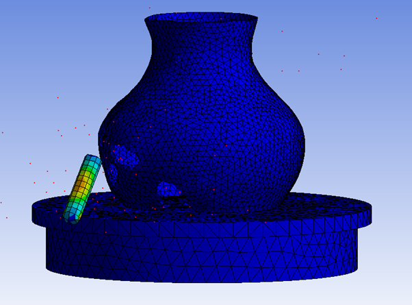
The last criterion is the On Minimum Element Time Step erosion. This is a very crude way of controlling the minimum time step by simply removing the elements which would otherwise yield a smaller computational time step than desired. By default, the Retain Inertia of Eroded Material is set to Yes. This allows you to examine the erosion process and follow the debris distribution (the defaults are different for Low Velocity and Quasi Static simulation types). An example of eroded material can be seen in the following figure.

Figure 8.15: Example of Eroded Material in a Model Simulating a Bullet going Through a Vase (eroded elements colored red)

Sometimes, especially when highly flexible materials are present, constant frequency oscillations can arise in the Explicit simulation. This can be avoided by the use of Static Damping. A damping value is calculated by dividing double the time step by the longest period of oscillation in the system. In other words, this value should be aimed at damping the slowest vibration in the analysis. When you are not sure of the value that should be used, it is best to start from the smallest damping valude to prevent overdamping. If the simulation is underdamped there will still be vibration visible, but when the simulation is overdamped it can lead to longer end time requirement and skewing of results. The other damping controls should be left at their defaults.