


When using the Explicit solver to investigate a problem that was originally solved using the Implicit solver, you should set up the analysis to take advantage of the features unique to the Explicit solver. As discussed earlier, the Explicit simulation takes into account the inertial forces and one of its most important parameters is the solve time (not to be mistaken with the actual run time it takes for the model to solve). The Explicit simulation can be seen as a chunk of the real time of an event that is slowed down as if using a high speed camera. The time values that the Explicit solver usually works with are much smaller than 1 second. For these quasi-static Implicit to Explicit simulations, we are working with a total time of around one millisecond to 1 second.
As stated earlier, one of the main parameters governing the solution is the time. The End Time defines the time frame which the solver simulates, starting from zero going up to the End Time value. The End Time should match the last entry in any of the boundary conditions tabular data time setting. This is a good place to estimate the maximum velocity in the model—if there are any displacements or deformations, dividing the distance covered by the end time gives a good estimate for the initial run. An end time target would be between 0.001 seconds and 1 second for the quasi-static simulations. Typically the explicit models are constrained by the end time so the Maximum Number of Cycles should be left at the default value or set to a very large number (for example, 1E7).
Each cycle is a piece of the solution time with the length of the current timestep and it is the constraint for a single iteration. It has a variable time value depending on the settings and the events during the solve so it is by no means guaranteed to be consistent. The maximum cycle number is rarely used to control the solution in explicit dynamics. Its most common use is when you need to do a short solution to check something in the setup and the Maximum Number of Cycles is set to a very small value (10,100,1000 etc). Even if we calculate the exact number of cycles we need and we have set a time step value, it is always better to use the end time to determine when the solve will terminate.
The timestep is the time increment at which the solve advances, and the solve time between two calculation cycles. The smaller the timestep is and the more complex the calculations per cycle are (dense mesh, material models etc.) the longer run time the solution will take. Having control over the timestep is crucial for achieving an effective simulation. There are numerous ways to keep track of and control the timestep. The governing factor for the timestep value is the smallest mesh element size and its mass. The timestep is calculated based on sound speed (which depends on density and material properties) and it needs to have a small enough value to accurately simulate the stress waves traveling through the body.
The following equation is used to determine the minimum timestep:

where  is the timestep safety factor (usually not changed from default value),
 is the element characteristic dimension (determined by smallest element size)
and
is the element characteristic dimension (determined by smallest element size)
and  is the sound speed in the material (depending on density and
elasticity).
is the sound speed in the material (depending on density and
elasticity).
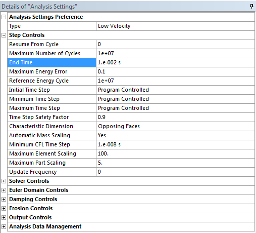
The initial, minimum, and maximum time step values usually should
be left as default (Program Controlled), except in a few cases. The Minimum Time
Step value is sometimes set to a very small number to allow the solve to continue
to run and not abort with the message: Time step too small.
You would set the Minimum Time Step like this when the time step is expected to become much
smaller than its initial value during the solve due to large deformations or complex contact.
When you set the value, this overrides the minimum time step conditions determined by the
solver, based on the initial setup. This user-defined minimum time step value might lead to a
much longer analysis run time.
Another case where user input might be required is when the analysis time step is determined by an element of a rigid body. A reasonably smaller time step should be used to prevent the simulation going forward using too large steps and becoming unstable. This can be achieved by a user defined Maximum Time Step value.
Figure 8.14: Default Solution Information display during solve with the estimated time remaining highlighted in yellow
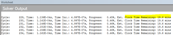
When you view the Solution Information while the solve is running, the Est. Clock Time Remaining can be observed. This is an new concept if you've only previously used the Implicit solver. This value gives an estimate of the remaining time needed to finish the solution. After the initial few cycles, and providing there are no abnormal deformations and unexpected events in the model during the solve, this value is quite accurate. It is based upon the time needed to calculate each cycle and the expected remaining number of cycles.
Usually when dealing with hyperelastic materials with a lot of deformation or other special cases, this remaining time will get a lot higher once the part of the simulation dealing with the large deformations is reached. This estimated time is also a good way to judge how changes to the mesh and setup will affect the solution time. After each change the model can be solved until a certain cycle number then interrupted, and the estimated time can be compared. This gives a rough estimate since it does not take into account any possible difficulties which might arise, but it is a useful tool for comparison.
As discussed earlier, the simulation will create a number of restart files that can be used to resume the solve following an interruption. There are a few things to consider when restarting a simulation. First, you have to make sure that the run will restart from the correct point. Set the Resume From Cycle value, which is based on the cycle number rather than simulation time. Another thing to note is that the boundary conditions cannot be altered before restarting and if, for example, the end time is extended and the user wants to continue the run, all of boundary conditions will assume they are kept constant at the last value of the normal solve time (before the time extension). Any change made to the setup while the solve is interrupted will mean that the restart is no longer possible. You must be careful when examining the interrupted solve results.