Even though both solvers model structural problems, the boundary conditions have a number of differences. Unlike the Explicit dynamic structural solver, the Implicit static structural solver has no real dependency on inertia. That is why the load cases in Implicit are usually 1 second per step, which is an arbitrary amount. Altering this value does not really have any effect on the solution. The Explicit Dynamics solver, on the other hand, uses time as its main reference for the calculations since the duration of the events in an Explicit problem are extremely short, and it is one of the most important aspects of the solve. When the two systems are connected and use the same Mechanical instance, boundary conditions can be copied by dragging and dropping from the Implicit to the Explicit system. This is the initial step in transferring the boundary conditions, but before the Explicit solve, adjustments to the boundary condition definitions must be made.
Unlike the Explicit solver, the Implicit solver has no real dependency on inertia (in the static structural solver). That is why the load cases in Implicit are usually 1 second per step, which is an arbitrary amount. Altering this value does not really have any effect on the solution. The Explicit Dynamics solver, on the other hand, uses time as its main reference for the calculations since the duration of the events in an Explicit problem are extremely short, and it is one of the most important aspects of the solve (see Timestep Controls).
As a starting point, a time scale factor of 100 or 1000 should be used; that is, 1 second in the implicit solver becomes 1E-2 or 1E-3 seconds in the explicit solver. The main thing to monitor are the velocities in the model. A good velocity to aim for is 5 m/s; it is not too low going into the static setup realm and it is not too high which would introduce significant inertial effects.
There are a few Mechanical boundary conditions that do not exist in Explicit Dynamics. Some of them can be simulated by using other boundary conditions. These include cylindrical support, frictionless support, bolt pretension and others. Refer to the table below for ways to simulate some of the missing boundary conditions.
| Boundary condition | Implicit solver | Explicit solver |
| Frictionless support | Available |
Available/ Simulated by using an equivalent symmetry plane (rigid behavior) or by creating displacement with fixed components to provide the desired constraint. |
| Bolt pretension | Available |
Pre-stress the bolt by using load steps:
|
| Cylindrical support | Available | Simulated using remote displacement to restrict rotation. |
| Displacement (step applied) | Available | Simulated using different boundary conditions to give the same movement - force, velocity etc. |
| Pressure (tabular variable value) | Available | Simulated using the Magnitude - Function setting to create a function giving the same values across the scoped geometry. |
When the scoping of two (or more) boundary conditions is done on two (or more) intersecting planes, the constraints on the shared edge (node) may trigger an error. The Explicit solver will only allow more than one boundary condition to be applied to the same edge in the following scenarios. Note that each of the following scenarios is evaluated for each of the load steps defined under analysis settings.
Both boundary conditions are defined on the same coordinate system and the combination of constraints do not conflict.
Both boundary conditions are defined on mutually orthogonal cartesian coordinate systems and the combination of constraints do not conflict.
Both boundary conditions are defined on cylindrical coordinate systems whose z-axes are aligned with one another and the combination of constraints do not conflict.
Both boundary conditions are defined on cartesian coordinate systems that have one axis aligned (and the constraints in the two boundary conditions in that direction do not conflict) but the other two do not. This scenario is depicted in Figure 1 where the y axis in CS1 is parallel to the y axis in CS2. Then the allowed constraints in the remaining axes x and z in both CS1 and CS2 are:
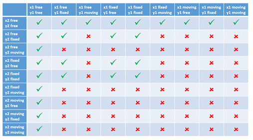
If the x and z constraints in one boundary condition are both free (then there are no restrictions on the constraints in x and z on the other boundary condition).
Where all of the constraints in x and z in both boundary conditions are either fixed or free
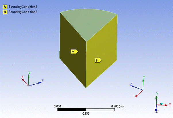
Figure depicting two boundary conditions whose scoping shares a common edge and that are defined on coordinate systems that are not orthogonal. BoundaryCondition1 is defined on the coordinate system (CS1) shown on the left. BoundaryCondition2 is defined on the coordinate system (CS2) shown on the right. CS1 and CS2 both have their y axes aligned, but the x in CS1 is not orthogonal to x in CS2, and z in CS1 is not orthogonal to z in CS2.
When the two coordinate systems share one axis in the same direction and the other two sets of two axes are not aligned, the constraints allowed on these remaining four axes are those shown in the table below marked with green checkmark.
Note:
Two functions that are the same function but are expressed using a different string (including differences in white space) may cause conflicts which cannot be resolved by the Explicit Dynamics solver (although they are not technically conflicting constraints).
The check for conflicting boundary conditions becomes more stringent if multiple load steps are defined under analysis settings and one (or more) of these boundary conditions is deactivated during the analysis. An additional conflict may exist if the solver is not able to combine the active and deactivated boundary condition into a single new boundary condition and apply it to the common nodes. An error along the following lines will be given, followed by a suggestion to circumvent the conflict:
The coordinate systems of two boundary conditions are compatible (or incompatible) but a deactivated load step causes the values of the boundary conditions to conflict. <suggestion>
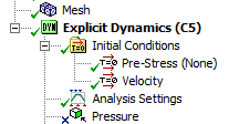
The Initial Conditions object in the Explicit Dynamics system can be helpful when certain aspects of the Implicit model cannot be directly recreated. It is a simple initial velocity, angular or directional, that is scoped to a body and is assigned at the initial cycle. This can be altered freely by different boundary conditions and events during the solve; its value is not constrained or limited. Another use for Initial Conditions is adding a pre-stress, usually from an Implicit solve. This is useful when an extensive complex combined simulation is required, and is not intended for situations where you need to run the same model setup with the two different solvers.