


Included in this section:
EnSight6 Wild Card Name Specification
EnSight6 Per_Node Variable File Format
EnSight6 Per_Element Variable File Format
EnSight6 Measured/Particle File Format
EnSight6 data consists of the following files:
Case (required) (points to all other needed files including model geometry, variables, and possibly measured geometry and variables)
EnSight6 supports constant result values as well as scalar, vector, 2nd order symmetric tensor, and complex variable fields.
EnSight makes no assumptions regarding the physical significance of the variable values in the files. These files can be from any discipline. For example, the scalar file can include such things as pressure, temperature, and stress. The vector file can be velocity, displacement, or any other vector data. And so on.
All variable results for EnSight6 are contained in disk files - one variable per file. Additionally, if there are multiple time steps, there must either be a set of disk files for each time step (transient multiple-file format), or all time steps of a particular variable or geometry in one disk file (transient single-file format). Thus, all EnSight6 transient geometry and variable files can be expressed in either multiple file format or single file format.
Sources of EnSight6 data include the following:
Data that can be translated to conform to the EnSight6 data format
Data that originates from one of the translators supplied with the EnSight application
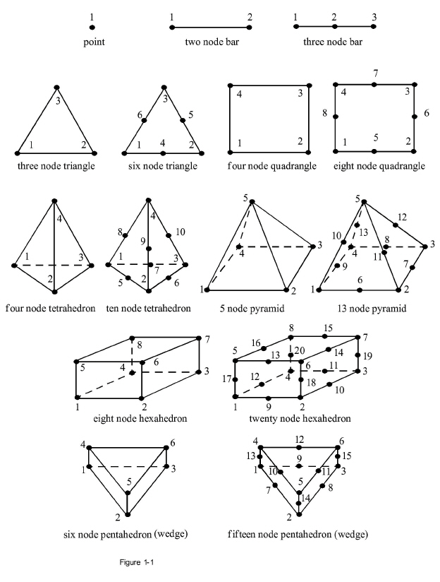
The EnSight6 format supports an unstructured defined element set as shown in the figure on the following page. Unstructured data must be defined in this element set. Elements that do not conform to this set must either be subdivided or discarded. The EnSight6 format also supports a structured block data format which is very similar to the PLOT3D format. For the structured format, the standard order of nodes is such that I's advance quickest, followed by J's, and then K's. A given EnSight6 model may have either unstructured data, structured data, or a mixture of both.
ens_checker
A program is supplied with EnSight which attempts to verify the integrity of the format of EnSight6 and EnSight Gold files. If you are producing EnSight formatted data, this program can be very helpful, especially in your development stage, in making sure that you are adhering to the published format. It makes no attempt to verify the validity of floating point values, such as coordinates, variable values, etc. This program takes a casefile as input. Thus, it will check the format of the casefile, and all associated geometry and variable files referenced in the casefile. See Use ens_checker.
The elements that are supported by the EnSight6 format are:
The Case file is an ASCII free format file that contains all the file and name information for accessing model (and measured) geometry, variable, and time information. It is comprised of five sections (FORMAT, GEOMETRY, VARIABLE, TIME, FILE) as described below:
Note: All lines in the Case file are limited to 79
The titles of each section must be in all capital letters.
Anything preceded by a # denotes a comment and is ignored. Comments may append information lines or be placed on their own lines.
Information following ":" may be separated by white spaces or tabs.
Specifications encased in "[ ]" are optional, as indicated.
Format Section
This is a required section which specifies the type of data to be read.
Usage:
FORMAT
type: ensight
Geometry Section
This is a required section which specifies the geometry information for the model (as well as measured geometry if present, and periodic match file Periodic Matchfile Format if present).
Usage:
GEOMETRY
model:         [ts] [fs]         filename [change_coords_only]
measured:      [ts] [fs]         filename [change_coords_only]
match:                           filename
boundary:                        filename
where: ts = time set number as
specified in TIME section. This is optional.
fs = corresponding file set number
as specified in FILE section below.
filename = The filename of the
appropriate file.
→ Model or measured filenames for a static geometry case, as well as match and boundary filenames will not contain "*" wildcards.
→ Model or measured filenames for a changing geometry case will contain "*" wildcards.
change_coords_only = The option to
indicate that the changing geometry (as indicated by wildcards in the filename) is
coords only.
Otherwise, changing geometry connectivity will be assumed.
Variable Section
This is an optional section which specifies the files and names of the variables. Constant variable values can also be set in this section.
Usage:
VARIABLE
constant per case:            [ts]         description  const_value(s)
scalar per node:              [ts] [fs]    description  filename
vector per node:              [ts] [fs]    description  filename
tensor symm per node:         [ts] [fs]    description  filename
scalar per element:           [ts] [fs]    description  filename
vector per element:           [ts] [fs]    description  filename
tensor symm per element:      [ts] [fs]    description  filename
scalar per measured node:     [ts] [fs]    description  filename
vector per measured node:     [ts] [fs]    description  filename
complex scalar per node:      [ts] [fs]    description  Re_fn   Im_fn   freq
complex vector per node:      [ts] [fs]    description  Re_fn   Im_fn   freq
complex scalar per element:   [ts] [fs]    description  Re_fn   Im_fn   freq
complex vector per element:   [ts] [fs]    description  Re_fn   Im_fn   freq
Note: Only transient filenames contain "*" wildcards.
Re_fn = The filename for the file
containing the real values of the complex variable.
Im_fn = The filename for the file
containing the imaginary values of the complex variable.
freq = The corresponding harmonic frequency of the complex
variable. For complex variables where harmonic frequency is undefined, simply use
the text string: UNDEFINED.
Note: As many variable description lines as needed may be used.
Variable descriptions have the following restrictions:
The maximum variable name length is documented at the beginning of this chapter.
Duplicate variable descriptions are not allowed.
Leading and trailing white space will be eliminated.
Variable descriptions must not start with a numeric digit.
Variable descriptions must not contain any of the following reserved:
' '
'!'
'@'
'#'
'$'
'^'
'('
')'
'['
']'
'*'
'/'
'+'
'-'
','
'.'
''
'\\'
'\''
'"'
'<'
'>'
'?'
'|'
Time Section
This is an optional section for steady state cases, but is required for transient cases. It contains time set information. Shown below is information for one time set. Multiple time sets (up to 16) may be specified for measured data as shown in Case File Example 3 below.
Usage:
TIME
time set:                 ts [description]
number of steps:          ns
filename start number:    fs
filename increment:       fi
time values:              time_1 time_2 .... time_ns
or
TIME
time set:                 ts [description]
number of steps:          ns
filename numbers:         fn
time values:              time_1 time_2 .... time_ns
where: ts = timeset
number. This is the number referenced in the GEOMETRY
and VARIABLE sections.
description = optional timeset description
which will be shown in user
interface.
ns = number of transient steps
fs = the number to replace the "*" wildcards in
the filenames, for the first step
fi = the increment to fs for subsequent
steps
time = the actual time values for each step,
each of which must be separated by a white space and which may continue on the next
line if needed
fn = a list of numbers or indices, to replace
the "*" wildcards in the filenames.
File Section
This section is optional for expressing a transient case
with single-file formats. This section contains single-file set information. This
information specifies the number of time steps in each file of each data entity, i.e. each geometry and
each variable (model and/or measured). Each data entity's corresponding file set
might have multiple
continuation files due to system file size limit, i.e. ~2 GB for -bit
and ~4 TB for 64-bit architectures. Each file set corresponds to one and only one
time set, but a time set may be referenced by many file sets. The following
information may be specified in each file set. For file sets where all of the time
set data exceeds the maximum file size limit of the system, both filename index and number of steps are repeated within the file set definition for each
continuation file required. Otherwise filename
index may be omitted if there is only one file. File set information is
shown in Example 10.19: Case File Example 4.
Usage:
FILE
file set:                 fs
filename index:           fi # Note: only used when data continues in other files
number of steps:          ns
where: fs = file set
number. This is the number referenced in the GEOMETRY
and VARIABLE sections above.
ns = number of transient steps
fi = file index number in the file name
(replaces * in the filenames)
Example 10.16: Case File Example 1
The following is a minimal EnSight6 case file for a steady state model with some results.
Note: This (en6.case) file, as well as all of its referenced geometry and variable files (along with a couple of command files) can be found under your installation directory (path: $CEI/ensight242/data/user_manual). The EnSight6 Geometry File Example and the Variable File Examples are the contents of these files.
FORMAT
type:  ensight
GEOMETRY
model:  en6.geo
VARIABLE
constant per case:            Cden  .8

scalar per element:           Esca  en6.Esca
scalar per node:              Nsca  en6.Nsca

vector per element:           Evec  en6.Evec
vector per node:              Nvec  en6.Nvec

tensor symm per element:      Eten  en6.Eten
tensor symm per node:         Nten  en6.Nten

complex scalar per element:   Ecmp  en6.Ecmp_r en6.Ecmp_i   2.
complex scalar per node:      Ncmp  n6.Ncmp_r en6.Ncmp_i    4.
Example 10.17: Case File Example 2
The following is a Case file for a transient model. The connectivity of the geometry is also changing.
FORMAT
type:  ensight

GEOMETRY
model:               1                   example2.geo**

VARIABLE
scalar per node:     1    Stress          example2.scl**
vector per node:     1    Displacement    example2.dis**

TIME
time set:                    1
number of steps:             3
filename start number:       0
filename increment:          1
time values:     1.0   2.0   3.0
The following files would be needed for Example 2:
example2.geo00     example2.scl00     example2.dis00
example2.geo01     example2.scl01     example2.dis01
example2.geo02     example2.scl02     example2.dis02
Example 10.18: Case File Example 3
The following is a Case file for a transient model with measured data.
This example has pressure given per element.
FORMAT
type:  ensight
GEOMETRY
model:                1              example3.geo*
measured:             2              example3.mgeo**


VARIABLE
constant per case:                     Gamma            1.4
constant per case:                1    Density          .9 .9 .7 .6 .6
scalar per element                1    Pressure         example3.pre*
vector per node:                  1    Velocity         example3.vel*
scalar per measured node:         2    Temperature      example3.mtem**
vector per measured node:         2    Velocity         example3.mvel**

TIME
time set:                   1
number of steps:            5
filename start number:      1
filename increment:         2
time values:                .1 .2 .3         # This example shows that time
.4 .5           # values can be on multiple lines
time set:                   2
number of steps:            6
filename start number:      0
filename increment:         2
time values:
.05 .15 .25 .34 .45 .55
The following files would be needed for Example 3:
example3.geo1         example3.pre1         example3.vel1
example3.geo3         example3.pre3         example3.vel3
example3.geo5         example3.pre5         example3.vel5
example3.geo7         example3.pre7         example3.vel7
example3.geo9         example3.pre9         example3.vel9
example3.mgeo00       example3.mtem00       example3.mvel00
example3.mgeo02       example3.mtem02       example3.mvel02
example3.mgeo04       example3.mtem04       example3.mvel04
example3.mgeo06       example3.mtem06       example3.mvel06
example3.mgeo08       example3.mtem08       example3.mvel08
example3.mgeo10       example3.mtem10       example3.mvel10
Example 10.19: Case File Example 4
The following is Example 10.18: Case File Example 3 expressed in transient single-file formats.
In this example, the transient data for the measured velocity data entity happens to be greater than the maximum file size limit. Therefore, the first four time steps fit and are contained in the first file, and the last two time steps are 'continued' in a second file.
FORMAT
type: ensight
GEOMETRY
model:               1    example4.geo
measured:            2    example4.mgeo

VARIABLE
constant per case:                     Density         .5
scalar per element:          1    1    Pressure        example4.pre
vector per node:             1    1    Velocity        example4.vel
scalar per measured node:    2    2    Temperature     example4.mtem
vector per measured node:    2    3    Velocity        example4.mvel*

TIME
time set:              1    Model
number of steps:       5
time values:          .1 .2 .3 .4 .5
time set:              2    Measured
number of steps:       6
time values:          .05 .15 .25 .34 .45 .55
FILE
file set:              1
number of steps:       5
file set:              2
number of steps:       6
file set:              3
filename index:        1
number of steps:       4
filename index:        2
number of steps:       2
The following files would be needed for Example 4:
example4.geo         example4.pre         example4.vel
example4.mgeo        example4.mtem        example4.mvel1
                                          example4.mvel2
Contents of TransientSingle Files
Each file contains transient data that corresponds to the specified number of time steps.
The data for each time step sequentially corresponds to the
simulation time values (time values) found
listed in the TIME section. In transient single-file format, the data for each time
step essentially corresponds to a standard EnSight6 geometry or variable file (model
or measured) as expressed in multiple file format. The data for each time step is
enclosed between two wrapper records, i.e. preceded by a BEGIN TIME STEP record and
followed by an END TIME STEP record. Time step data is not split between files. If
there is not enough room to append the data from a time step to the file without
exceeding the maximum file limit of a particular system, then a continuation file
must be created for the time step data and any subsequent time step. Any type of
user comments may be included before and/or after each transient step
wrapper.
Note: If transient single file format is used, EnSight expects all files of a dataset to be specified in transient single file format. Thus, even static files must be enclosed between a BEGIN TIME STEP and an END TIME STEP wrapper.
For binary geometry files, the first BEGIN TIME STEP wrapper must follow the <C Binary/Fortran Binary> line. Both BEGIN TIME STEP and END TIME STEP wrappers are written according to type (1) in binary, Writing EnSight6 Binary Files.
Efficient reading of each file (especially binary) is facilitated by appending each file with a file index. A file index contains appropriate information to access the file byte positions of each time step in the file. (EnSight automatically appends a file index to each file when exporting in transient single file format.) If used, the file index must follow the last END TIME STEP wrapper in each file.
File Index Usage:
|
ASCII |
Binary |
Item |
Description |
|
"%20d\n" |
sizeof(int) |
n |
Total number of data time steps in the file. |
|
"%20d\n" |
sizeof(long) |
fb1 |
File byte loc for contents of 1st time step* |
|
"%20d\n" |
sizeof(long) |
fb2 |
File byte loc for contents of 2nd time step* |
|
. . . |
. . . |
. . . |
. . . |
|
"%20d\n" |
sizeof(long) |
fbn |
File byte loc for contents of nth time step* |
|
"%20d\n" |
sizeof(int) |
flag |
Miscellaneous flag (= 0 for now) |
|
"%20d\n" |
sizeof(long) |
fb of item n |
File byte loc for Item n above |
|
"%s\n" |
sizeof(char)*80 |
"FILE_INDEX" |
File index keyword |
* Each file byte location is the first byte that follows the BEGIN TIME STEP record.
Shown below are the contents of each of the above files, using the data files from Case File Example 3 for reference (without FILE_INDEX for simplicity).
Contents of file example4.geo_1:
                                BEGIN TIME STEP
                                Contents of file example3.geo1
                                END TIME STEP
                                BEGIN TIME STEP
                                Contents of file example3.geo3
                                END TIME STEP
                                BEGIN TIME STEP
                                Contents of file example3.geo5
                                END TIME STEP
                                BEGIN TIME STEP
                                Contents of file example3.geo7
                                END TIME STEP
                                BEGIN TIME STEP
                                Contents of file example3.geo9
                                END TIME STEP
Contents of file example4.pre_1:
                                BEGIN TIME STEP
                                Contents of file example3.pre1
                                END TIME STEP
                                BEGIN TIME STEP
                                Contents of file example3.pre3
                                END TIME STEP
                                BEGIN TIME STEP
                                Contents of file example3.pre5
                                END TIME STEP
                                BEGIN TIME STEP
                                Contents of file example3.pre7
                                END TIME STEP
                                BEGIN TIME STEP
                                Contents of file example3.pre9
                                END TIME STEP
Contents of file example4.vel_1:
                                BEGIN TIME STEP
                                Contents of file example3.vel1
                                END TIME STEP
                                BEGIN TIME STEP
                                Contents of file example3.vel3
                                END TIME STEP
                                BEGIN TIME STEP
                                Contents of file example3.vel5
                                END TIME STEP
                                BEGIN TIME STEP
                                Contents of file example3.vel7
                                END TIME STEP
                                BEGIN TIME STEP
                                Contents of file example3.vel9
                                END TIME STEP
Contents of file example4.mgeo_1:
                                BEGIN TIME STEP
                                Contents of file example3.mgeo00
                                END TIME STEP
                                BEGIN TIME STEP
                                Contents of file example3.mgeo02
                                END TIME STEP
                                BEGIN TIME STEP
                                Contents of file example3.mgeo04
                                END TIME STEP
                                BEGIN TIME STEP
                                Contents of file example3.mgeo06
                                END TIME STEP
                                BEGIN TIME STEP
                                Contents of file example3.mgeo08
                                END TIME STEP
                                BEGIN TIME STEP
                                Contents of file example3.mgeo10
                                END TIME STEP
Contents of file example4.mtem_1:
                                BEGIN TIME STEP
                                Contents of file example3.mtem00
                                END TIME STEP
                                BEGIN TIME STEP
                                Contents of file example3.mtem02
                                END TIME STEP
                                BEGIN TIME STEP
                                Contents of file example3.mtem04
                                END TIME STEP
                                BEGIN TIME STEP
                                Contents of file example3.mtem06
                                END TIME STEP
                                BEGIN TIME STEP
                                Contents of file example3.mtem08
                                END TIME STEP
                                BEGIN TIME STEP
                                Contents of file example3.mtem10
                                END TIME STEP
Contents of file example4.mvel1_1:
                                BEGIN TIME STEP
                                Contents of file example3.mvel00
                                END TIME STEP
                                BEGIN TIME STEP
                                Contents of file example3.mvel02
                                END TIME STEP
                                BEGIN TIME STEP
                                Contents of file example3.mvel04
                                END TIME STEP
                                BEGIN TIME STEP
                                Contents of file example3.mvel06
                                END TIME STEP
Contents of file example4.mvel2_1:
                                Comments can precede the beginning wrapper here.
                                BEGIN TIME STEP
                                Contents of file example3.mvel08
                                END TIME STEP
                                Comments can go between time step wrappers here.
                                BEGIN TIME STEP
                                Contents of file example3.mvel10
                                END TIME STEP
Comments can follow the ending time step wrapper.For transient data, if multiple time files are involved, the file names must conform to the EnSight wild-card specification. This specification is as follows:
File names must include numbers that are in ascending order from beginning to end.
Numbers in the files names must be zero filled if there is more than one significant digit.
Numbers can be anywhere in the file name.
When the file name is specified in the EnSight result file, you must replace the numbers in the file with an asterisk(*). The number of asterisks specified is the number of significant digits. The asterisk must occupy the same place as the numbers in the file names.
The EnSight6 format consists of keywords followed by information. The following seven items are important when working with EnSight6 geometry files:
You do not have to assign node IDs. If you do, the element connectivities are based on the node numbers. If you let EnSight assign the node IDs, the nodes are considered to be sequential starting at node 1, and element connectivity is done accordingly. If node IDs are set to off, they are numbered internally; however, you will not be able to display or query on them. If you have node IDs in your data, you can have EnSight ignore them by specifying "node id ignore." Using this option may reduce some of the memory taken up by the Client and Server, but display and query on the nodes will not be available.
You do not need to specify element IDs. If you specify element IDs, or you let EnSight assign them, you can show them on the screen. If they are set to off, you will not be able to show or query on them. If you have element IDs in your data you can have EnSight ignore them by specifying "element id ignore." Using this option will reduce some of the memory taken up by the Client and Server. This may or may not be a significant amount, and remember that display and query on the elements will not be available.
The format of integers and real numbers must be followed (See the Geometry Example below).
Integers are written out using the following integer format:
From C:
8dformatFrom FORTRAN:
i8format
Real numbers are written out using the following floating-point format:
From C:
12.5eformatFrom FORTRAN:
e12.5format
The number of integers or reals per line must also be followed!
By default, a Part is processed to show the outside boundaries. This representation is loaded to the Client host system when the geometry file is read (unless other attributes have been set on the workstation, such as feature angle).
Coordinates for unstructured data must be defined before any Parts can be defined. The different elements can be defined in any order (that is, you can define a hexa8 before a bar2).
A Part containing structured data cannot contain any unstructured element types or more than one block. Each structured Part is limited to a single block. A structured block is indicated by following the Part description line with either the "block" line or the "block iblanked" line. An "iblanked" block must contain an additional integer array of values at each node, traditionally called the iblank array. Valid iblank values for the EnSight format are:
0 for nodes which are exterior to the model, sometimes called blanked-out nodes
1 for nodes which are interior to the model, thus in the free stream and to be used <0 or >1 for any kind of boundary nodes
In EnSight's structured Part building dialog, the iblank option selected will control which portion of the structured block is "created". Thus, from the same structured block, the interior flow field part as well as a symmetry boundary part could be "created".
Note: By default EnSight does not do any "partial" cell iblank processing. Namely, only complete cells containing no "exterior" nodes are created. It is possible to obtain partial cell processing by issuing the "test:partial_cells_on" command in the Command Dialog before reading the file.
Note: For the structured format, the standard order of nodes is such that I's advance quickest, followed by J's, and then K's.
Maximum number of parts is 32769Maximum number of variables is 10000Maximum file name length is 1024Maximum part name length is 79, but the GUI will only display 49Maximum variable name length is 79, but the GUI will only display 49
Generic Format
Not all of the lines included in the following generic example file are necessary:
description line 1                     |
description line 2                     |
node id <off/given/assign/ignore>      | All geometry files must element id
<off/given/assign/ignore>              | contain these first six lines coordinates
                                       |
# of unstructured nodes                |
id x y z
id x y z
id x y z
.
.
.
part #
description line
point
number of points
id nd
id nd
id nd
.
.
.
bar2
number of bar2’s
id nd nd
id nd nd
id nd nd
.
.
.
bar3
number of bar3’s
id nd nd nd
id nd nd nd
id nd nd nd
.
.
.
tria3
number of three node triangles

id nd nd nd
id nd nd nd
id nd nd nd
.
.
.
tria6
number of six node triangles
id nd nd nd nd nd nd
.
.
.
quad4
number of quad 4’s
id nd nd nd nd
id nd nd nd nd
id nd nd nd nd
id nd nd nd nd
.
.
.
quad8
number of quad 8’s
id nd nd nd nd nd nd nd nd
id nd nd nd nd nd nd nd nd
id nd nd nd nd nd nd nd nd
id nd nd nd nd nd nd nd nd
.
.
.
tetra4
number of 4 node tetrahedrons
id nd nd nd nd
id nd nd nd nd
id nd nd nd nd
id nd nd nd nd
.
.
.
tetra10
number of 10 node tetrahedrons
id nd nd nd nd nd nd nd nd nd nd
id nd nd nd nd nd nd nd nd nd nd
id nd nd nd nd nd nd nd nd nd nd
id nd nd nd nd nd nd nd nd nd nd
.
.
.
pyramid5
number of 5 node pyramids
id nd nd nd nd nd
id nd nd nd nd nd
id nd nd nd nd nd
id nd nd nd nd nd
.
.
.
pyramid13
number of 13 node pyramids
id nd nd nd nd nd nd nd nd nd nd nd nd nd
id nd nd nd nd nd nd nd nd nd nd nd nd nd
nd nd nd nd nd nd nd nd nd nd
id nd nd nd nd nd nd nd nd nd nd nd nd nd
.
.
.
hexa8
number of 8 node hexahedrons
id nd nd nd nd nd nd nd nd
id nd nd nd nd nd nd nd nd
id nd nd nd nd nd nd nd nd
id nd nd nd nd nd nd nd nd
.
.
.
hexa20
number of 20 node hexahedrons
id nd nd nd nd nd nd nd nd nd nd nd nd nd nd nd nd nd nd nd nd
id nd nd nd nd nd nd nd nd nd nd nd nd nd nd nd nd nd nd nd nd
id nd nd nd nd nd nd nd nd nd nd nd nd nd nd nd nd nd nd nd nd
id nd nd nd nd nd nd nd nd nd nd nd nd nd nd nd nd nd nd nd nd
id nd nd nd nd nd nd nd nd nd nd nd nd nd nd nd nd nd nd nd nd
.
.
.
penta6
number of 6 node pentahedrons
id nd nd nd nd nd nd
id nd nd nd nd nd nd
id nd nd nd nd nd nd
id nd nd nd nd nd nd
id nd nd nd nd nd nd
.
.
.
penta15
number of 15 node pentahedrons
id nd nd nd nd nd nd nd nd nd nd nd nd nd nd nd
id nd nd nd nd nd nd nd nd nd nd nd nd nd nd nd
id nd nd nd nd nd nd nd nd nd nd nd nd nd nd nd
id nd nd nd nd nd nd nd nd nd nd nd nd nd nd nd
id nd nd nd nd nd nd nd nd nd nd nd nd nd nd nd
.
.
.
part #
description line
block                                     #nn=i*j*k
        i       j      k
x_n1 x_n2 x_n3 ..... x_nn                 (6/line)
y_n1 y_n2 y_n3 ..... y_nn                 “
z_n1 z_n2 z_n3 ..... z_nn                 “

part #
description line
block iblanked                             #nn=i*j*k i j k
x_n1 x_n2 x_n3 ..... x_nn                 (6/line)
y_n1 y_n2 y_n3 ..... y_nn                 “
z_n1 z_n2 z_n3 ..... z_nn                 “
ib_n1 ib_n2 ib_n3 .... ib_nn             (10/line)
EnSight6 Geometry File Example
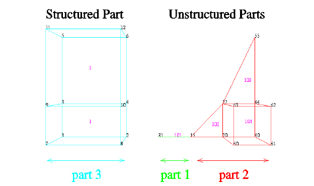
The following is an example of an ASCII EnSight6 geometry file with 11 defined unstructured nodes from which 2 unstructured parts are defined, and a 2x3x2 structured part as depicted in the above diagram. (See Case File Example 1 for reference to this file.)
This is the 1st description line of the EnSight6 geometry example This is the 2nd description line of the EnSight6 geometry example node id given
element id given coordinates
11
15 4.00000e+00 0.00000e+00 0.00000e+00
31 3.00000e+00 0.00000e+00 0.00000e+00
20 5.00000e+00 0.00000e+00 0.00000e+00
40 6.00000e+00 0.00000e+00 0.00000e+00
22 5.00000e+00 1.00000e+00 0.00000e+00
44 6.00000e+00 1.00000e+00 0.00000e+00
55 6.00000e+00 3.00000e+00 0.00000e+00
60 5.00000e+00 0.00000e+00 2.00000e+00
61 6.00000e+00 0.00000e+00 2.00000e+00
62 6.00000e+00 1.00000e+00 2.00000e+00
63 5.00000e+00 1.00000e+00 2.00000e+00

part 1
2D uns-elements (description line for
part 1) tria3


        2


        102	15	20	22
        103	22	44	55
hexa8
        1

104 20 40 44 22 60 61 62
                                                        63
part 2
1D uns-elements (description line for
part 2) bar2

    1
    101 31 15
part 3
3D struct-part (description line for part 3)
block iblanked
2 3 2
0.00000e+00 2.00000e+00 0.00000e+00 2.00000e+00 0.00000e+00 2.00000e+00
0.00000e+00 2.00000e+00 0.00000e+00 2.00000e+00 0.00000e+00 2.00000e+00
0.00000e+00 0.00000e+00 1.00000e+00 1.00000e+00 3.00000e+00 3.00000e+00
0.00000e+00 0.00000e+00 1.00000e+00 1.00000e+00 3.00000e+00 3.00000e+00
0.00000e+00 0.00000e+00 0.00000e+00 0.00000e+00 0.00000e+00 0.00000e+00
2.00000e+00 2.00000e+00 2.00000e+00 2.00000e+00 2.00000e+00 2.00000e+00
1 1 1 1 1 1 1 1 1 1
EnSight6 variable files can either be per_node or per_element. They cannot be both. However, an EnSight model can have some variables which are per_node and other variables which are per_element.
EnSight6 variable files for per_node variables contain any values for each unstructured node followed by any values for each structured node.
First comes a single description line.
Second comes any unstructured node value. The number of values per node depends on the type of field. An unstructured scalar field has one, a vector field has three (order: x,y,z), a 2nd order symmetric tensor field has 6 (order: 11, 22, 33, 12, 13, 23), and a 2nd order asymmetric tensor field has 9 values per node (order: 11, 12, 13, 21, 22, 23, 31,, 33). An unstructured complex variable in EnSight6 consists of two scalar or vector fields (one real and one imaginary), with scalar and vector values written to their separate files respectively.
Third comes any structured data information, starting with a part # line, followed by a line containing the "block", and then lines containing the values for each structured node which are output in the same IJK component order as the coordinates. Briefly, a structured scalar is the same as an unstructured scalar, one value per node. A structured vector is written one value per node per component, thus three sequential scalar field blocks. Likewise for a structured 2nd order symmetric tensor, written as six sequential scalar field blocks, and a 2nd order tensor, written as nine sequential scalar field blocks. The same methodology applies for a complex variable only with the real and imaginary fields written to separate structured scalar or vector files.
The values must be written in the following floating point format ( 6 per line as shown in the examples below):
From C: 12.5e
format
From FORTRAN: e12.5
format
The format of a per_node variable file is as follows:
Line 1
This line is a description line.
Line 2 through the end of the file contains the values at each node in the model.
A generic example for per_node variables:
One description line for the entire file
*.*****E+** *.*****E+** *.*****E+** *.*****E+** *.*****E+** *.*****E+**
*.*****E+** *.*****E+** *.*****E+** *.*****E+** *.*****E+** *.*****E+**
*.*****E+** *.*****E+** *.*****E+** *.*****E+**
part #
block
*.*****E+** *.*****E+** *.*****E+** *.*****E+** *.*****E+** *.*****E+**
*.*****E+** *.*****E+**
*.*****E+** *.*****E+** *.*****E+** *.*****E+** *.*****E+** *.*****E+**
*.*****E+** *.*****E+**
*.*****E+** *.*****E+** *.*****E+** *.*****E+** *.*****E+** *.*****E+**
*.*****E+** *.*****E+**
Note: There is a format difference between the unstructured and structured (block) portions of the vector and tensor data. For example a multiple component unstructured vector appears as x y z triplets, while the structured counterpart lists all x then all y and finally all z.
The following variable file examples reflect scalar, vector, tensor, and complex variable values per node for the previously defined EnSight6 Geometry File Example with 11 defined unstructured nodes and a 2x3x2 structured Part (Part number 3). The values are summarized in the following table.
|
|
|||||||
|
|
|
|
|
|
|
|
|
|
|
|
|
|
|
|
|
|
|
Unstructured |
|||||||
|
1 |
15 |
(1.) |
(1.1, 1.2, 1.3) |
(1.1, 1.2, 1.3, 1.4, 1.5, 1.6) |
(1.1) |
(1.2) |
|
|
2 |
31 |
(2.) |
(2.1, 2.2, 2.3) |
(2.1, 2.2, 2.3, 2.4, 2.5, 2.6) |
(2.1) |
(2.2) |
|
|
3 |
20 |
(3.) |
(3.1, 3.2, 3.3) |
(3.1, 3.2, 3.3, 3.4, 3.5, 3.6) |
(3.1) |
(3.2) |
|
|
4 |
40 |
(4.) |
(4.1, 4.2, 4.3) |
(4.1, 4.2, 4.3, 4.4, 4.5, 4.6) |
(4.1) |
(4.2) |
|
|
5 |
22 |
(5.) |
(5.1, 5.2, 5.3) |
(5.1, 5.2, 5.3, 5.4, 5.5, 5.6) |
(5.1) |
(5.2) |
|
|
6 |
44 |
(6.) |
(6.1, 6.2, 6.3) |
(6.1, 6.2, 6.3, 6.4, 6.5, 6.6) |
(6.1) |
(6.2) |
|
|
7 |
55 |
(7.) |
(7.1, 7.2, 7.3) |
(7.1, 7.2, 7.3, 7.4, 7.5, 7.6) |
(7.1) |
(7.2) |
|
|
8 |
60 |
(8.) |
(8.1, 8.2, 8.3) |
(8.1, 8.2, 8.3, 8.4, 8.5, 8.60 |
(8.1) |
(8.2) |
|
|
9 |
61 |
(9.) |
(9.1, 9.2, 9.3) |
(9.1, 9.2, 9.3, 9.4, 9.5, 9.6) |
(9.1) |
(9.2) |
|
|
10 |
62 |
(10.) |
(10.1,10.2,10.3) |
(10.1,10.2, 10.3,10.4, 10.5,10.6) |
(10.1) |
(10.2) |
|
|
11 |
63 |
(11.) |
(11.1,11.2,11.3) |
(11.1,11.2, 11.3,11.4, 11.5,11.6) |
(11.1) |
(11.2) |
|
|
Structured |
|||||||
|
1 |
1 |
(1.) |
(1.1, 1.2, 1.3) |
(1.1, 1.2, 1.3, 1.4, 1.5, 1.6) |
(1.1) |
(1.2) |
|
|
2 |
2 |
(2.) |
(2.1, 2.2, 2.3) |
(2.1, 2.2, 2.3, 2.4, 2.5, 2.6) |
(2.1) |
(2.2) |
|
|
3 |
3 |
(3.) |
(3.1, 3.2, 3.3) |
(3.1, 3.2, 3.3, 3.4, 3.5, 3.6) |
(3.1) |
(3.2) |
|
|
4 |
4 |
(4.) |
(4.1, 4.2, 4.3) |
(4.1, 4.2, 4.3, 4.4, 4.5, 4.6) |
(4.1) |
(4.2) |
|
|
5 |
5 |
(5.) |
(5.1, 5.2, 5.3) |
(5.1, 5.2, 5.3, 5.4, 5.5, 5.6) |
(5.1) |
(5.2) |
|
|
6 |
6 |
(6.) |
(6.1, 6.2, 6.3) |
(6.1, 6.2, 6.3, 6.4, 6.5, 6.6) |
(6.1) |
(6.2) |
|
|
7 |
7 |
(7.1, 7.2, 7.3) |
(7.1, 7.2, 7.3, 7.4, 7.5, 7.6) |
(7.1) |
(7.2) |
||
|
8 |
8 |
(8.) |
(8.1, 8.2, 8.3) |
(8.1, 8.2, 8.3, 8.4, 8.5, 8.6) |
(8.1) |
(8.2) |
|
|
9 |
9 |
(9.) |
(9.1, 9.2, 9.3) |
(9.1, 9.2, 9.3, 9.4, 9.5, 9.6) |
(9.1) |
(9.2) |
|
|
10 |
10 |
(10.) |
(10.1,10.2,10.3) |
(10.1,10.2, 10.3,10.4,
10.5,10.6) |
(10.1) |
(10.2) |
|
|
11 |
11 |
(11.) |
(11.1,11.2,11.3) |
(11.1,11.2, 11.3,11.4,
11.5,11.6) |
(11.1) |
(11.2) |
|
Per_node (Scalar) Variable Example 1
This example shows ASCII scalar file (en6.Nsca) for the geometry example.
Per_node scalar values for the EnSight6 geometry example
 1.00000E+00 2.00000E+00 3.00000E+00 4.00000E+00 5.00000E+00 6.00000E+00
 7.00000E+00 8.00000E+00 9.00000E+00 1.00000E+01 1.10000E+01
part 3
block
 1.00000E+00 2.00000E+00 3.00000E+00 4.00000E+00 5.00000E+00 6.00000E+00
 7.00000E+00 8.00000E+00 9.00000E+00 1.00000E+01 1.10000E+01
Per_node (Vector) Variable Example 2
This example shows ASCII vector file (en6.Nvec) for the geometry example.
Per_node vector values for the EnSight6 geometry example
 1.10000E+00 1.20000E+00 1.30000E+00 2.10000E+00 2.20000E+00 2.30000E+00
 3.10000E+00 3.20000E+00 3.30000E+00 4.10000E+00 4.20000E+00 4.30000E+00
 5.10000E+00 5.20000E+00 5.30000E+00 6.10000E+00 6.20000E+00 6.30000E+00
 7.10000E+00 7.20000E+00 7.30000E+00 8.10000E+00 8.20000E+00 8.30000E+00
 9.l0000E+00 9.20000E+00 9.30000E+00 1.01000E+01 1.02000E+01 1.03000E+01
 1.11000E+01 1.12000E+01 1.13000E+01
part 3
block
 1.10000E+00 2.10000E+00 3.10000E+00 4.10000E+00 5.10000E+00 6.10000E+00
 7.10000E+00 8.10000E+00 9.10000E+00 1.01000E_01 1.11000E+01
 1.20000E+00 2.20000E+00 3.20000E+00 4.20000E+00 5.20000E+00 6.20000E+00
 7.20000E+00 8.20000E+00 9.20000E+00 1.02000E+01 1.12000E+01
 1.30000E+00 2.30000E+00 3.30000E+00 4.30000E+00 5.30000E+00 6.30000E+00
 7.30000E+00 8.30000E+00 9.30000E+00 1.03000E+01 1.13000E+01
Per_node (Tensor) Variable Example 3
This example shows an ASCII 2nd order symmetric tensor file (en6.Nten) for the geometry example.
Per_node symmetric tensor values for the EnSight6 geometry example
 1.10000E+00 1.20000E+00 1.30000E+00 1.40000E+00 1.50000E+00 1.60000E+00
 2.10000E+00 2.20000E+00 2.30000E+00 2.40000E+00 2.50000E+00 2.60000E+00
 3.10000E+00 3.20000E+00 3.30000E+00 3.40000E+00 3.50000E+00 3.60000E+00
 4.10000E+00 4.20000E+00 4.30000E+00 4.40000E+00 4.50000E+00 4.60000E+00
 5.10000E+00 5.20000E+00 5.30000E+00 5.40000E+00 5.50000E+00 5.60000E+00
 6.10000E+00 6.20000E+00 6.30000E+00 6.40000E+00 6.50000E+00 6.60000E+00
 7.10000E+00 7.20000E+00 7.30000E+00 7.40000E+00 7.50000E+00 7.60000E+00
 8.10000E+00 8.20000E+00 8.30000E+00 8.40000E+00 8.50000E+00 8.60000E+00
 9.10000E+00 9.20000E+00 9.30000E+00 9.40000E+00 9.50000E+00 9.60000E+00
 1.01000E+01 1.02000E+01 1.03000E+01 1.04000E+01 1.05000E+01 1.06000E+01
 1.11000E+01 1.12000E+01 1.13000E+01 1.14000E+01 1.15000E+01 1.16000E+01
part 3
block
 1.10000E+00 2.10000E+00 3.10000E+00 4.10000E+00 5.10000E+00 6.10000E+00
 7.10000E+00 8.10000E+00 9.10000E+00 1.01000E+01 1.11000E+01
 1.20000E+00 2.20000E+00 3.20000E+00 4.20000E+00 5.20000E+00 6.20000E+00
 7.20000E+00 8.20000E+00 9.20000E+00 1.02000E+01 1.12000E+01
 1.30000E+00 2.30000E+00 3.30000E+00 4.30000E+00 5.30000E+00 6.30000E+00
 7.30000E+00 8.30000E+00 9.30000E+00 1.03000E+01 1.13000E+01
 1.40000E+00 2.40000E+00 3.40000E+00 4.40000E+00 5.40000E+00 6.40000E+00
 7.40000E+00 8.40000E+00 9.40000E+00 1.04000E+01 1.14000E+01
 1.50000E+00 2.50000E+00 3.50000E+00 4.50000E+00 5.50000E+00 6.50000E+00
 7.50000E+00 8.50000E+00 9.50000E+00 1.05000E+01 1.15000E+01
 1.60000E+00 2.60000E+00 3.60000E+00 4.60000E+00 5.60000E+00 6.60000E+00
 7.60000E+00 8.60000E+00 9.60000E+00 1.06000E+01 1.16000E+01
Per_node (Complex) Variable Example 4
This example shows the ASCII complex real (en6.Ncmp_r) and imaginary (en6.Ncmp_i) scalar files for the geometry example. (The same methodology would apply for complex real and imaginary vector files.)
Real scalar File:
Per_node complex real scalar values for the EnSight6 geometry example
 1.10000E+00 2.10000E+00 3.10000E+00 4.10000E+00 5.10000E+00 6.10000E+00
 7.10000E+00 8.10000E+00 9.10000E+00 1.01000E+01 1.11000E+01
part 3
block
 1.10000E+00 2.10000E+00 3.10000E+00 4.10000E+00 5.10000E+00 6.10000E+00
 7.10000E+00 8.10000E+00 9.10000E+00 1.01000E+01 1.11000E+01 1.21000E+00
Imaginary scalar File:
Per_node complex imaginary scalar values for the EnSight6 geometry example
 1.20000E+00 2.20000E+00 3.20000E+00 4.20000E+00 5.20000E+00 6.20000E+00
 7.20000E+00 8.20000E+00 9.20000E+00 1.02000E+01 1.12000E+01
part 3
block
 1.20000E+00 2.20000E+00 3.20000E+00 4.20000E+00 5.20000E+00 6.20000E+00
 7.20000E+00 8.20000E+00 9.20000E+00 1.02000E+01 1.12000E+01 1.22000E+00
EnSight variable files for per_element variables contain values for each element of designated types of designated Parts. First comes a single description line. Second comes a Part line. Third comes an element type line and fourth comes the value for each element of that type and part. If it is a scalar variable, there is one value per element, while for vector variables there are three values per element. (The number of elements of the given type are obtained from the corresponding EnSight6 geometry file.)
The values must be written in the following floating point format (6 per line as shown in the examples below):
From C: 12.5e
format
From FORTRAN: e12.5
format
The format of a per_element variable file is as follows:
Line 1 This line is a description line.
Line 2 Part line, with part number corresponding to the geometry file.
Line 3 Element type line ( example: tria3, hexa8, ... )
Line 4 Repeats until next element type line, part line, or end of file is reached. Lists values for each element of this part and type.
A generic example for per_element variables:
One description line for the entire file
part #
element type
 *.*****E+** *.*****E+** *.*****E+** *.*****E+** *.*****E+** *.*****E+**
 *.*****E+** *.*****E+**
part #
block
 *.*****E+** *.*****E+** *.*****E+** *.*****E+** *.*****E+** *.*****E+**
 *.*****E+** *.*****E+** *.*****E+** *.*****E+**
 *.*****E+** *.*****E+** *.*****E+** *.*****E+** *.*****E+** *.*****E+**
 *.*****E+** *.*****E+** *.*****E+** *.*****E+**
 *.*****E+** *.*****E+** *.*****E+** *.*****E+** *.*****E+** *.*****E+**
 *.*****E+** *.*****E+** *.*****E+** *.*****E+**
Note: There is a format difference between the unstructured and structured (block) portions of the vector and tensor data. For example a multiple component unstructured vector appears as x y z triplets, while the structured counterpart lists all x then all y and finally all z.
The following variable file examples reflect scalar, vector, tensor, and complex variable values per element for the previously defined EnSight6 Geometry File Example with 11 defined unstructured nodes and a 2x3x2 structured Part (Part number 3). The values are summarized in the following table.
|
Complex Scalar |
|||||||
|
Element |
Element |
Scalar |
Vector |
Tensor (2nd order symm.) |
Real |
Imaginary |
|
|
Index |
Id |
Value |
Values |
Values |
Value |
Value |
|
|
Unstructured |
|||||||
|
bar2 |
|||||||
|
1 |
101 |
(1.) |
(1.1, 1.2, 1.3) |
(1.1, 1.2, 1.3, 1.4, 1.5, 1.6) |
(1.1) |
(1.2) |
|
|
tria3 |
|||||||
|
1 |
102 |
(2.) |
(2.1, 2.2, 2.3) |
(2.1, 2.2, 2.3, 2.4, 2.5, 2.6) |
(2.1) |
(2.2) |
|
|
2 |
103 |
(3.) |
(3.1, 3.2, 3.3) |
(3.1, 3.2, 3.3, 3.4, 3.5, 3.6) |
(3.1) |
(3.2) |
|
|
hexa8 |
|||||||
|
1 |
104 |
(4.) |
(4.1, 4.2, 4.3) |
(4.1, 4.2, 4.3, 4.4, 4.5, 4.6) |
(4.1) |
(4.2) |
|
|
Structured |
|||||||
|
block |
1 |
1 |
(5.) |
(5.1, 5.2, 5.3) |
(5.1, 5.2, 5.3, 5.4, 5.5, 5.6) |
(5.1) |
(5.2) |
|
2 |
2 |
(6.) |
(6.1, 6.2, 6.3) |
(6.1, 6.2, 6.3, 6.4, 6.5, 6.6) |
(6.1) |
(6.2) |
|
|
3 |
3 |
(7.) |
(7.1, 7.2, 7.3) |
(7.1, 7.2, 7.3, 7.4, 7.5, 7.6) |
(7.1) |
(7.2) |
|
|
4 |
4 |
(8.) |
(8.1, 8.2, 8.3) |
(8.1, 8.2, 8.3, 8.4, 8.5, 8.6) |
(8.1) |
(8.2) |
|
|
5 |
5 |
(9.) |
(9.1, 9.2, 9.3) |
(9.1, 9.2, 9.3, 9.4, 9.5, 9.6) |
(9.1) |
(9.2) |
|
|
6 |
6 |
(10.) |
(10.1, 10.2, 10.3) |
(10.1, 10.2, 10.3, 10.4, 10.5, 10.6) |
(10.1) |
(10.2) |
|
|
7 |
7 |
(11.) |
(11.1, 11.2, 11.3) |
(11.1, 11.2, 11.3, 11.4, 11.5, 11.6) |
(11.1) |
(11.2) |
|
|
8 |
8 |
(12.) |
(12.1, 12.2, 12.3) |
(12.1, 12.2, 12.3, 12.4, 12.5, 12.6) |
(12.1) |
(12.2) |
|
Per_element (Scalar) Variable Example 1
This example shows an ASCII scalar file (en6.Esca) for the geometry example.
Per_elem scalar values for the EnSight6 geometry example
part 1
tria3
 2.00000E+00 3.00000E+00
hexa8
 4.00000E+00
part 2
bar2
 1.00000E+00
part 3
block
 5.00000E+00 6.00000E+00 7.00000E+00 8.00000E+00 9.00000E+00 1.00000E+01
 1.10000E+01 1.20000E+01
Per_element (Vector) Variable Example 2
This example shows an ASCII vector file (en6.Evec) for the geometry example.
Per_elem vector values for the EnSight6 geometry example
part 1
tria3
 2.10000E+00 2.20000E+00 2.30000E+00 3.10000E+00 3.20000E+00 3.30000E+00
hexa8
 4.10000E+00 4.20000E+00 4.30000E+00
part 2
bar2
 1.10000E+00 1.20000E+00 1.30000E+00
part 3
block
 5.10000E+00 6.10000E+00 7.10000E+00 8.10000E+00 9.10000E+00 1.01000E+01
 1.11000E+01 1.21000E+01
 5.20000E+00 6.20000E+00 7.20000E+00 8.20000E+00 9.20000E+00 1.02000E+01
 1.12000E+01 1.22000E+01
 5.30000E+00 6.30000E+00 7.30000E+00 8.30000E+00 9.30000E+00 1.03000E+01
 1.13000E+01 1.23000E+01
Per_element (Tensor) Variable Example 3 This example shows the ASCII 2nd order symmetric tensor file (en6.Eten) for the geometry example.
Per_elem symmetric tensor values for the EnSight6 geometry example
part 1
tria3
 2.10000E+00 2.20000E+00 2.30000E+00 2.40000E+00 2.50000E+00 2.60000E+00
 3.10000E+00 3.20000E+00 3.30000E+00 3.40000E+00 3.50000E+00 3.60000E+00
hexa8
 4.10000E+00 4.20000E+00 4.30000E+00 4.40000E+00 4.50000E+00 4.60000E+00
part 2
bar2
 1.10000E+00 1.20000E+00 1.30000E+00 1.40000E+00 1.50000E+00 1.60000E+00
part 3
block
 5.10000E+00 6.10000E+00 7.10000E+00 8.10000E+00 9.10000E+00 1.01000E+01
 1.11000E+01 1.21000E+01
 5.20000E+00 6.20000E+00 7.20000E+00 8.20000E+00 9.20000E+00 1.02000E+01
 1.12000E+01 1.22000E+01
 5.30000E+00 6.30000E+00 7.30000E+00 8.30000E+00 9.30000E+00 1.03000E+01
 1.13000E+01 1.23000E+01
 5.40000E+00 6.40000E+00 7.40000E+00 8.40000E+00 9.40000E+00 1.04000E+01
 1.14000E+01 1.24000E+01
 5.50000E+00 6.50000E+00 7.50000E+00 8.50000E+00 9.50000E+00 1.05000E+01
 1.15000E+01 1.25000E+01
 5.60000E+00 6.60000E+00 7.60000E+00 8.60000E+00 9.60000E+00 1.06000E+01
 1.16000E+01 1.26000E+01
Per_element (Complex) Variable Example 4
This example shows the ASCII complex real (en6.Ecmp_r) and imaginary (en6.Ecmp_i) scalar files for the geometry example. (The same methodology would apply for complex real and imaginary vector files).
Real scalar File:
Per_elem complex real scalar values for the EnSight6 geometry example
part 1
tria3
 2.10000E+00 3.10000E+00
hexa8
 4.10000E+00
part 2
bar2
 1.10000E+00
part 3
block
 5.10000E+00 6.10000E+00 7.10000E+00 8.10000E+00 9.10000E+00 1.01000E+01
 1.11000E+01 1.21000E+01
Imaginary scalar File:
Per_elem complex imaginary scalar values for the EnSight6 geometry example
part 1
tria3
 2.20000E+00 3.20000E+00
hexa8
 4.20000E+00
part 2
bar2
 1.20000E+00
part 3
block
 5.20000E+00 6.20000E+00 7.20000E+00 8.20000E+00 9.20000E+00 1.02000E+01
 1.12000E+01 1.22000E+01
The format of a Measured/Particle geometry file is exactly the same as an EnSight 5 measured/particle geometry file and is repeated below as follows:
Line 1
This line is a description line.
Line 2
Indicates that this file contains particle coordinates. The words "particle coordinates" should be entered on this line without the quotes.
Line 3
Specifies the number of Particles.
Line 4 through the end of the file.
Each line contains the ID and the X, Y, and Z coordinates of each Particle. The format of this line is "integer real real real" written out in the following format:
From C: %8d%12.5e%12.5e%12.5e format
From FORTRAN: i8,
3e12.5 format
A generic measured/Particle geometry file is as follows:
A description line
particle coordinates
#_of_Particles
id xcoord ycoord zcoord
id xcoord ycoord zcoord
id xcoord ycoord zcoord
.
.
.
Measured Geometry Example
The following illustrates a measured/Particle file with seven points:
This is a simple measured geometry file
particle coordinates
        7
       101 0.00000E+00 0.00000E+00 0.00000E+00
       102 1.00000E+00 0.00000E+00 0.00000E+00
       103 1.00000E+00 1.00000E+00 0.00000E+00
       104 0.00000E+00 1.00000E+00 0.00000E+00
       205 5.00000E-01 0.00000E+00 2.00000E+00
       206 5.00000E-01 1.00000E+00 2.00000E+00
       307 0.00000E+00 0.00000E+00-1.50000E+00
Measured Variable Files
Measured variable files use the same format as EnSight6
per_node variable files, which is exactly the same as the
EnSight 5 measured/particle variable files.
This section describes the EnSight6 binary files. This format is used to increase the speed of reading data into EnSight.
For binary files, there is a header that designates the type of binary file. This header is: C Binary or Fortran Binary. This must be the first thing in the geometry file only. The format for the file is then essentially the same format as the ASCII format, with the following exceptions:
The ASCII format puts the node and element ids on the same "line" as the corresponding coordinates. The BINARY format writes all node id's then all coordinates.
The ASCII format puts all element id's of a type within a Part on the same line as the corresponding connectivity. The BINARY format writes all the element ids for that type, then all the corresponding connectivities of the elements.
FORTRAN binary files should be created as sequential access unformatted files.
Float arrays (such as coordinates and variable values) must be single precision. Double precision is not supported.
In all the descriptions of binary files that follow, the number on the left end of the line corresponds to the type of write of that line, according to the following code:
This is a write of 80 to the file:
C example:
char buffer[80];
strcpy(buffer,”C Binary”);
fwrite(buffer,sizeof(char),80,file_ptr);
FORTRAN:
character*80 buffer
buffer = “Fortran Binary”
write(10) buffer
This is a write of a single integer:
C example:
fwrite(&num_nodes,sizeof(int),1,file_ptr);
FORTRAN:
write(10) num_nodes
This is a write of an integer array:
C example:
C example: fwrite(node_ids,sizeof(int),num_nodes,file_ptr);
FORTRAN:
FORTRAN:write(10) (node_ids(i),i=1,num_nodes)
This is a write of a float array:
C example:
fwrite(coords,sizeof(float),3*num_nodes,file_ptr);
FORTRAN:
write(10) ((coords(i,j),i=1,3),j=1,num_nodes)
Note: For EnSight6 format, when using Fortran binary, and writing arrays composed of components, such as coordinates, or vector values, it is very important that they all be written with a single Fortran write statement. If you instead were to write the coords in the statement above with a loop per component, such that the write statement is executed three times, like the following, EnSight will not be able to read it!
FORTRAN: do 200 i=1,3
write(10) (coords(i,j),j=1,num_nodes)
200 continue
EnSight6 Binary Geometry
An EnSight binary geometry file contains information in the following order:
(1) <C Binary/Fortran Binary>
(1) description line 1
(1) description line 2
(1) node id <given/off/assign/ignore>
(1) element id <given/off/assign/ignore>
(1) coordinates
(2) #_of_points
(3) [point_ids]
(4) coordinate_array (For FORTRAN make sure only one write statement is used)
(1) part #
(1) description line
(1) element_type
(2) #_of_element_type
(3) [element_ids] for the element_type
(3) connectivities for the element_type
(1) element_type
(2) #_of_element_type
(3) [element_ids] for the element_type
(3) connectivities for the element_type
:
(1) part #
(1) description line
(1) element_type
(2) #_of_element_type
(3) [element_ids] for the element_type
(3) connectivities for the element_type
(1) element_type
(2) #_of_element_type
(3) [element_ids] for the element_type
(3) connectivities for the element_type
(1) part #
(1) description line
(1) block [iblanked]
(3) i j k
(4) all i coords, all j coords, all k coords (For FORTRAN make sure only one write statement is used)
(3) [iblanking]
:
Per_node Binary Scalar
An EnSight6 binary scalar file contains information in the following order:
(1) description line
(4) scalar_array for unstructured nodes
(1) part #
(1) block
(4) scalar_array for part's structured nodes
Per_node Binary Vector
An EnSight6 binary vector file contains information in the following order:
(1) description line
(4) vector_array for unstructured nodes (For FORTRAN make sure only one write statement is used)
(1) part #
(1) block
(4) vector_array for part's structured nodes (For FORTRAN make sure only one write statement is used)
Per_node Binary Tensor
An EnSight6 binary tensor file contains information in the following order:
(1) description line
(4) tensor_array for unstructured nodes (For FORTRAN make sure only one write statement is used)
(1) part #
(1) block
(4) tensor_array for part's structured nodes (For FORTRAN make sure only one write statement is used)
Per_node Binary Complex
An EnSight6 binary complex real and imaginary scalar files contain information in the following order: (The same methodology applies for the complex real and imaginary vector files.)
Real scalar file:
(1) description line
(4) real scalar_array for unstructured nodes
(1) part #
(1) block
(4) real scalar_array for part's structured nodes
Imaginary scalar file:
(1) description line
(4) imaginary scalar_array for unstructured nodes
(1) part #
(1) block
(4) imaginary scalar_array for part's structured nodes
Per_element Binary Scalar
An EnSight6 binary scalar file contains information in the following order:
(1) description line
(1) part #
(1) element type (tria3, quad4, ...)
(4) scalar_array for elements of part and type
(1) part #
(1) block
(4) scalar_array for structured elements of part
Per_element Binary Vector
An EnSight6 binary vector file contains information in the following order:
(1) description line
(1) part #
(1) element type (tria3, quad4, ...)
(4) vector_array for elements of part and type (For FORTRAN make sure only one write statement is used)
(1) part #
(1) block
(4) vector_array for structured elements of part (For FORTRAN make sure only one write statement is used)
Per_element Binary Tensor
An EnSight6 binary tensor file contains information in the following order:
(1) description line
(1) part #
(1) element type (tria3, quad4, ...)
(4) tensor_array for unstructured elements of part and type (For FORTRAN make sure only one write statement is used)
(1) part #
(1) block
(4) tensor_array for structured elements of part and type (For FORTRAN make sure only one write statement is used)
Per_element Binary Complex
EnSight6 binary complex real and imaginary scalar files contain information in the following order: (The same methodology applies for the complex real and imaginary vector files.)
Real scalar file:(1) description line(1) part #(1) element type (tria3, quad4, ...)(4) real scalar_array for unstructured elements of part and type(1) part #(1) block(4) real scalar_array for structured elements of part and type
Imaginary scalar file:(1) description line(1) part #(1) element type (tria3, quad4, ...)(4) imaginary scalar_array for unstructured elements of part and type(1) part #(1) block(4) imaginary scalar_array for structured elements of part and type
Binary Measured Geometry
An EnSight6 binary measured/particle geometry file contains information in the following order:
(1) <C Binary/Fortran Binary>
(1) description line 1
(1) particle coordinates
(2) #_of_points
(3) point_ids
(4) coordinate_array (For FORTRAN make sure only one write statement is used)
Binary Measured Variable Files
EnSight6 binary measured/discrete particle scalar and vector files follow the same binary formats as EnSight6 model per-node scalar and vector files.