


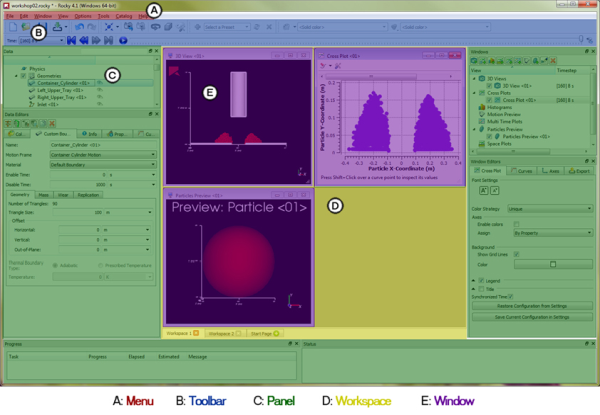
Rocky is a powerful program with a flexible, hierarchical interface. One main screen gives you access to the most frequently used functions and features, and provides you with various views of the simulation.
Additional panels allow you to access properties and settings to fine-tune your simulation and view statistics based upon the results.
What would you like to learn about?
See Also:
Use this section to explore the five major parts of the Rocky user interface, and learn when and why you might access them.
What would you like to do?
Learn more About the Menu
Learn more About the Toolbar
Learn more About Panels
Learn more About Workspaces
See Also:
The menu is always located at the very top of the Rocky main screen and is one of the few UI elements in Rocky that is static in its location. From the Rocky menu, you can do all of the following tasks:
From the File menu:
Begin a new simulation project (see also Begin a New Simulation Project).
Open an existing simulation project (see also Open an Existing Simulation Project).
Save a new simulation project (see also Save a New Simulation Project).
Archive a simulation project (see also Archive a Simulation Project).
Restore an archived project (see also Restore an Archived Simulation Project).
Export or import project context (see also Reuse 3D View Window, Workspace, and User Process Setups in Other Projects).
From the Edit menu:
Undo or Redo actions made in Rocky (see also About the Undo/Redo History Panel).
Copy an Image or Data Set to the clipboard (see also Copy an Image or Data Set to the Clipboard).
From the Window menu, you can create, organize (see also Edit or Remove a Workspace), and save an image of (see also Save an Image of the 3D View, Plot, or Histogram) various Rocky windows, including:
3D View windows (see also Create and Modify a 3D View).
Plot and Histogram windows (see also Graphing (Plot or Histogram) a Data Set Within Rocky).
Motion Preview windows (see also Preview a Motion in 3D).
Particles Details windows (see also Preview a Particle Shape in 3D).
From the View menu:
Show/hide various Rocky panels (see also About Panels).
Revert to the default Rocky user interface layout by clicking Reset layout.
Change the background color of the Rocky interface by selecting a Theme. In this version, there are two options:
Light Theme (default), which has a mostly white background with dark-colored text.
Dark Theme, which has a mostly black background with light-colored text.
From the Options menu:
Set global preferences for using Rocky (see also About Setting Global Preferences).
Set the units used in Rocky (see also About Setting Your Unit System).
Install coupling components required for use with Ansys Fluent (see also Install Ansys Coupling Components).
From the Tools menu, you can show/hide all of the following panels:
The PrePost Script panel (see also About Creating and Using PrePost Scripts).
The Inspection panel (see also About the Cell Inspector).
The Animation panel (see also About Creating and Saving an Animation).
The Python Shell panel (see also Customize and Extend Rocky with Python).
The Expressions/Variables panel (see also Defining Your Variables).
From the Help menu, you can do all of the following:
Access your Rocky License status and info by clicking License Info.
Review details about this Rocky release by clicking About. (See also About This Version of Rocky.)
Access the User Manual (this document), DEM Technical Manual, and other resources by pointing to Manuals and then selecting which option you want. (See also Getting Help and Support.)
Access the Tutorials, Community forum and other features by pointing to Customer Portal and then selecting which item you want.
Review the technical library, the latest Rocky applications and other resources by pointing to Website and then clicking the option you want to access.
Learn about the key improvements made for this release of Rocky by clicking What's New.
Review what changed in this release of Rocky by clicking Changelog.
Access the default Workspace that displays when you first open Rocky by clicking Start Page.
See Also:
The toolbar is, by default, located at the top of the Rocky main screen just below the menu. There are several individual toolbar components that can make up the main Rocky toolbar, including the following:
Camera visualization toolbar (see also About Using the Camera Visualization Toolbar)
Coloring service toolbar (see also About Using the Coloring Service Toolbar to Change a 3D View)
Custom Presets toolbar (see also About the Custom Presets Toolbar)
File toolbar
Time toolbar (see also About the Time Toolbar)
Undo Redo toolbar
These individual toolbar components can be moved or made to float independent of the screen by clicking a toolbar handle and then dragging it and dropping it with the mouse. You can also show/hide individual toolbars by right clicking a toolbar and selecting or clearing the options at the very bottom of the contextual menu.
See Also:
Below the toolbar and surrounding the Workspace are various floating panels that enable you to set parameters and choose options for your simulation and its resulting data. The primary panels for configuring your simulation are the Data and Data Editors panels that appear (by default) to the left of the Workspace; the primary panels for post-processing are the Windows and Windows Editors panels that appear (by default) to the right of the Workspace. Also showing (by default) to the right of the Workspace, you can display various tools panels such as Animations or PrePost Script. You can choose to show/hide multiple panels through both the View and Tools menus located at the top of the screen.
All panels in Rocky can be resized, moved, nested with other panels, and undocked to float independent of the Rocky main screen. Specifically:
To resize a panel, hover your mouse over a panel boundary until the resize icon appears. Then, click and drag the boundary to the desired width or height.
To move a panel to another docked location, click the panel title and drag to the desired area outside of the Workspace. While still dragging the panel, a preview of new docked locations will be displayed with a blue background. To select a new docked location, release the mouse over the preview of the location you want.
To make a nested panel, click the panel title and then drag it directly over another panel until the lower panel is blue, and then release the mouse. The second panel will appear as a tab at the bottom of the first panel. Select the tab you want to toggle between panels.
To make a docked panel float, click the panel title, drag it towards the center of the screen then release the mouse. Alternatively, you can also click the icon to the left of the panel's close button to make any docked panel float.
Show/hide multiple panels by right clicking a panel's title bar and selecting or clearing the options at the top and middle of the contextual menu.
What would you like to do?
Learn more About the Data Panel
Learn more About the Data Editors Panel
Learn more About the Windows Panel
Learn more About the Window Editors Panel
Learn more About the Undo/Redo History Panel
Learn more About the Log Panel
Learn more About the Simulation Log Panel
Learn more About the Cache Panel
Learn more About the Debug Info Panel
Learn more About the Progress Panel
Learn more About the Status Panel
Learn more About the PrePost Script Panel
Learn more About the Inspector Panel
Learn more About the Animations Panel
Learn more About the Python Shell Panel
Learn more About the Expressions/Variables Panel
See Also:
The Data panel is the area you use to select the entity with which you want to interact. The tree-like structure is hierarchical and is roughly organized by the steps required to setup, process, and analyze your project. (See Figure 1.)
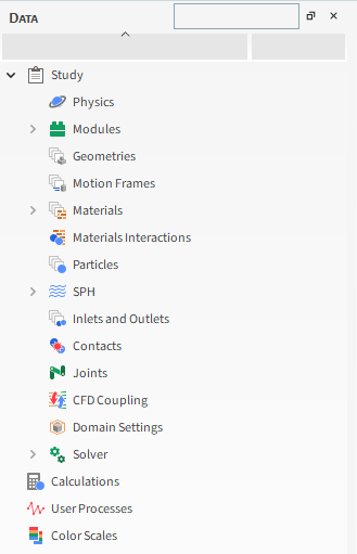
The top-level items in the Data panel include the following entities:
Study, which organizes all the various set-up and processing categories. (See also Set Simulation Parameters and Processing a Simulation.)
Particles Calculations, which lists any Particles Properties you have applied to User Processes for which you want to retain calculations after the particle leaves the defined area. (See also About Particles Calculations.)
User Processes, which lists the shapes, planes, and settings you have divided or filtered your simulation area into for more focused analysis. (See also Filter Views and Data with User Processes.)
Color Scales, which lists all the Properties you have shown in a 3D View for the purpose of changing the coloration of the legends. (See also Create and Modify a 3D View.)
Once selected in the Data panel, options for the item are generally shown in the Data Editors panel (see also About the Data Editors Panel), or through the item's right-click menu. Note: With the exception of the Study item, which has its own settings, top-level Data panel items are for categorization only and do not have settings associated with them. Only the sub-items listed beneath these categories will have settings upon which you can take action.
The Data panel also includes a search box to help you find items in the panel quickly. (See also Use the Data Panel Search Bar to Quickly Find Components.) You may also duplicate many of the items in the Data panel to save time on setup. (See also Duplicate a Data Panel Item.)
See Also:
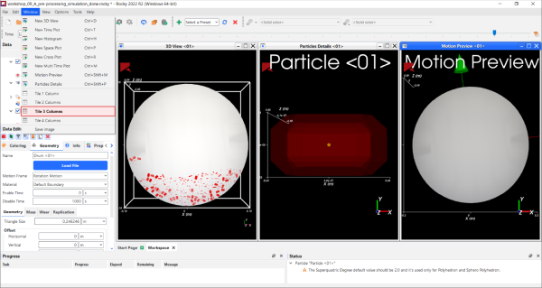
The Data Editors panel shows the settings and parameters available for the item selected in the Data panel (see also About the Data Panel). Figure 1 shows the Data Editors panel view when Particles is chosen in the Data panel.
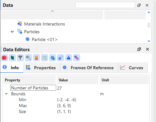
What is shown for an entity on the Data Editors panel can include action buttons, like those provided at the top of Figure 1, and settings and information organized into various tabs, such as the following:
Coloring tab (see also About the Coloring Tab)
Info tab (see also About the Info Tab)
Properties tab (see also About Properties)
Frames of Reference tab (see also About Creating Frames of Reference for Particles)
Curves tab (see also About Curves)
Some entities in the Data panel, such as Particles Calculations and Color Scales, are categories only and will have no information displayed in the Data Editors panel. However, sub-items within these categories will have information upon which you can take action.
See Also:
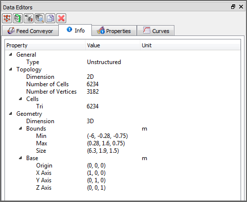
The Info tab is one of several tabs that appear on the Data Editors panel when a simulation entity is selected in the Data panel. Though purely informational, the Info tab does show some data about the selected entity that could be useful when setting up or analyzing your simulation.
For example, the Info tab can display domain properties, such as the topology and geometry coordinate limits, that provide context as to how the Property simulation data was recorded. These properties are displayed on the Info tab for simulation entities including conveyors (Figure 1) and imported geometries, the main Particles entity, 1-Way LBM, 1-Way Fluent, and individual User Processes.
The Info tab on individual Modules (see also About Modules Parameters) describes the Author and Version details for the Module, and lists what other entities in the Rocky UI are affected by enabling that particular Module. For example, the Info tab for the Liquid Bridge Model Module (Figure 2) describes three places in the Rocky UI affected by that module.
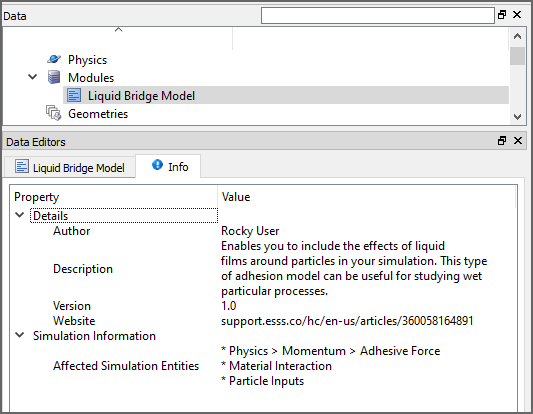
Note: In this version of Rocky, the Liquid Bridge Model Module is provided as an external module. Refer to the Install an External Module topic for details.
This information can help you verify that the parameters in those locations are set correctly for the feature enabled by the module.
When an individual Particle set is selected under the main Particles entity, the Info tab shows useful information about the largest particle in the selected particle set, but also contains additional functionality unique to that tab (Figure 3).
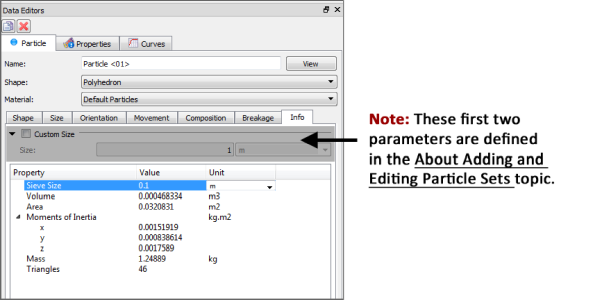
For example, you can change the units by clicking a unit and selecting a new type from the list that appears. You can also use the Custom Size (Custom Diameter or Custom Scale Factor) checkbox to experiment with different particle sizes and how they affect the properties displayed on the Info tab without having to switch back to the Size tab. Note: This functionality is explained in more detail in the About Adding and Editing Particle Sets topic.
The Max Admissible Overlap value is provided only for custom (imported) concave particles. Its purpose is to display the maximum percentage of concave overlap that will be allowed during the simulation.
As a comparison, for a sphere and a boundary collision, the maximum overlap allowed is 50%— above that the sphere center would be on the other side of the boundary and the particle would cross it. For concave particles, the maximum admissible overlap depends on the shape. Ideally, the maximum admissible overlap should not be too low, or you will have to compensate for that by using a larger Young's modulus for stability.
Tip: If you have imported a concave particle with values too small for the maximum overlap allowed, consider modifying the STL shape to result in higher values. This might help you avoid numerical issues.
Use the following information to help you better understand this value and how best to use it:
What is this value used for? It is a reference that can help you prevent excessive overlaps that can cause numerical instabilities for the concave particle shape used in the simulation. The smaller the maximum admissible overlap, the smaller are the overlap values that are tolerated during the simulation.
How is this value calculated? It is computed based upon the minimum distance from the particle's triangle centers to other triangles of the particle in the direction perpendicular to the triangle's plane. So the max admissible overlap is a function of the particle shape. Sharp edges will result in lower maximum admissible overlaps to guarantee the solver's stability.
How does this value relate to the STL file I imported? This is not a quality criteria for the STL file itself; rather, it is related to the particle shape. If the shape has more rounded or sharp edges, it will be reflected on the max admissible overlap value. So more (or fewer) overlaps will be admitted to ensure the stability of the simulations.
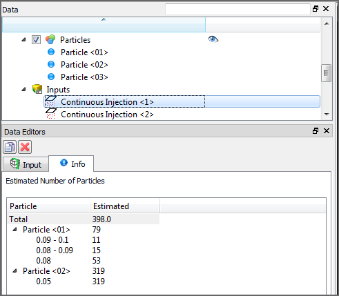
For Inputs (Figure 4), the Info tab displays the simulation particle count in different ways depending upon the particle size distribution that was specified:
For Particle sets made up of only one size (no size distribution), the Info tab shows the exact number of particles that will be released into the simulation.
For Particle sets with a size distribution, the Info tab provides an estimate of the number of particles that could be released into the simulation.
Note: For Volume Fill specifically, the estimate assumes there are no boundary limits to consider, and assumes a Gap Scale Factor equal to 1. This means that if you have set your particle Mass higher than the box and gap you define can contain, the particle estimate on the Info tab will show a higher number than what will actually be injected.
For Particle sets with size ranges specified, viewing the Simulation Summary after processing has begun is still the only place to get an exact particle count; however, if a particle count estimate is sufficient, the particle count on the Input entity's Info tab can be viewed at any time during project setup. (See also About the Simulation Summary.)
See tables below to help you understand more about the Info tab.
Table 1: Info tab definitions for individual Geometry components, Inlets, the main Particles entity, 1-Way LBM, 1-Way Fluent, and individual User Processes (Figure 1 above)
Property | Description | Values Displayed |
|---|---|---|
General | ||
Type | Indicates the type of grid the domain property is based upon. Specifically:
| Unstructured; Structured |
Topology | ||
Dimension | Indicates whether the domain property has no dimension; or is one dimensional (node), two dimensional (triangle), or three dimensional (block or cell). | 0D; 1D; 2D; 3D |
Number of Cells | Lists the number of cell within the simulation bounds. | Positive whole numbers |
Number of Vertices | The number of cell intersections within the simulation bounds. For geometries, this is the points between triangle. For Eulerian Statistics, this is the corner points making up each block And so on. | Positive whole numbers |
Cells Point | For Particles, lists the number of points within the simulation bounds. | Positive whole numbers |
Cells Tri | For Geometry components, lists the number of triangles within the simulation bounds. | Positive whole numbers |
Cells Bar | For Particle Trajectory calculations, lists the total number of trajectory bars that were calculated. | Positive whole numbers |
Shape | For Eulerian Statistics, indicates the number of divisions that were defined in the X, Y, and Z directions respectively. | Whole values greater than or equal to 1 |
Geometry | ||
Dimension | Indicates whether the geometry components within the simulation have no dimension; or are one dimensional (node), two dimensional (triangle), or three dimensional (block or cell). | 0D; 1D; 2D; 3D |
Bounds Min | The minimum coordinates of the simulation data. | X, Y, Z |
Bounds Max | The maximum coordinates of the simulation data. | X, Y, Z |
Bounds Size | The size dimensions of the current simulation bounds. | X, Y, Z |
Length | For Particle Trajectory calculations, provides the total length of the trajectory lines added together. | Positive values |
Volume | For Eulerian Statistics, provides the total volume of all the Eulerian blocks added together. | Positive values |
Table 2: Info tab definitions for individual Modules (Figure 2 above) (See also About Modules Parameters.)
Property | Description | Values Displayed |
|---|---|---|
Details | ||
Author | If provided, lists the name of the developer or company that designed and built the Module. | Text |
Description | If provided, displays a short description of what the Module does. | Text |
Version | If provided, displays the Module version. For Modules created by Ansys, this will be equal to the version of Rocky for which the Module was designed. | Text |
Website | If provided, displays the URL of the website associated with the Author of the Module. | Text |
Simulation Information | ||
Affected Simulation Entities | Describes whether or not enabling the Module caused changes or additional settings to be made in other areas of the Rocky UI. Specifically:
| Text |
Table 3: Info tab definitions for individual Particle sets (Figure 3 above) (See also About Adding and Editing Particle Sets.)
Property | Description | Values Displayed |
|---|---|---|
Scale Factor | By default, when the Custom Scale Factor checkbox is cleared, this displays the size of the largest particle in the Particle set using the Original Size Scale method of measurement that was selected on the Size sub-tab. When the Custom Scale Factor checkbox is enabled, this displays the experimental size entered in the corresponding Scale Factor) box. (See also About Adding and Editing Particle Sets.) | Positive values |
Equivalent Diameter | By default, when the Custom Diameter checkbox is cleared, this displays the size of the largest particle in the Particle set using the Equivalent Sphere Diameter method of measurement that is selected on the Size sub-tab. When the Custom Diameter checkbox is enabled, this displays the experimental size entered in the corresponding Diameter box. (See also About Adding and Editing Particle Sets.) | Positive values |
Sieve size | By default, when the Custom Size (Custom Diameter or Custom Scale Factor) checkbox is cleared, no matter what is selected for Size Type on the Size sub-tab, this converts the size of the largest particle to its Sieve Size value, which is based upon the dimensions of a square hole just big enough for the particle to pass through. When the Custom Size (Custom Diameter or Custom Scale Factor) checkbox is enabled, this displays the experimental size entered in the corresponding Size (Diameter or Scale Factor) box converted into its Sieve Size value. (See also About Adding and Editing Particle Sets.) | Positive values |
Volume | By default, when the Custom Size (Custom Diameter or Custom Scale Factor) checkbox is cleared, this displays the volume of the largest particle in the Particle set. When the Custom Size (Custom Diameter or Custom Scale Factor) checkbox is enabled, this displays the volume of the experimental particle defined in the corresponding Size (Diameter or Scale Factor) box. (See also About Adding and Editing Particle Sets.) | Positive values |
Area | By default, when the Custom Size (Custom Diameter or Custom Scale Factor) checkbox is cleared, this displays the surface area of the largest particle in the Particle set. When the Custom Size (Custom Diameter or Custom Scale Factor) checkbox is enabled, this displays the surface area of the experimental particle defined in the corresponding Size (Diameter or Scale Factor) box. (See also About Adding and Editing Particle Sets.) | Positive values |
Moments of Inertia x | By default, when the Custom Size (Custom Diameter or Custom Scale Factor) checkbox is cleared, this displays the moment of inertia in the X direction of the largest particle in the Particle set. When the Custom Size (Custom Diameter or Custom Scale Factor) checkbox is enabled, this displays the moment of inertia in the X direction for the experimental particle defined in the corresponding Size (Diameter or Scale Factor) box. (See also About Adding and Editing Particle Sets.) | Positive values |
Moments of Inertia y | By default, when the Custom Size (Custom Diameter or Custom Scale Factor) checkbox is cleared, this displays the moment of inertia in the Y direction of the largest particle in the Particle set. When the Custom Size (Custom Diameter or Custom Scale Factor) checkbox is enabled, this displays the moment of inertia in the Y direction for the experimental particle defined in the corresponding Size (Diameter or Scale Factor) box. (See also About Adding and Editing Particle Sets.) | Positive values |
Moments of Inertia z | By default, when the Custom Size (Custom Diameter or Custom Scale Factor) checkbox is cleared, this displays the moment of inertia in the Z direction of the largest particle in the Particle set. When the Custom Size (Custom Diameter or Custom Scale Factor) checkbox is enabled, this displays the moment of inertia in the Z direction for the experimental particle defined in the corresponding Size (Diameter or Scale Factor) box. (See also About Adding and Editing Particle Sets.) | Positive values |
Mass | By default, when the Custom Size (Custom Diameter or Custom Scale Factor) checkbox is cleared, this displays the mass of the largest particle in the Particle set. When the Custom Size (Custom Diameter or Custom Scale Factor) checkbox is enabled, this displays the mass of the experimental particle defined in the corresponding Size (Diameter or Scale Factor) box. (See also About Adding and Editing Particle Sets.) | Positive values |
Elements | For Particle sets with Multiple Elements selected on the Composition sub-tab, this displays the number of individual element that the particle shape will be divided into. Specifically:
(See also About Adding and Editing Particle Sets.) | Positive values |
Triangles | By default, when the Custom Size (Custom Diameter or Custom Scale Factor) checkbox is cleared, this displays the number of triangles that make up the largest particle in the Particle set. When the Custom Size (Custom Diameter or Custom Scale Factor) checkbox is enabled, this displays the number of triangles making up the experimental particle defined in the corresponding Size (Diameter or Scale Factor) box. (See also About Adding and Editing Particle Sets.) Note: The way in which particle shape triangles are counted in Rocky depend upon the particle shape and composition. Specifically:
| Positive values |
Vertices | For Particle sets made up of custom (imported) particle shapes, this displays the number of points between the triangle (for Custom Shells or Custom Polyhedrons) or between the segments (for Custom Fibers) that make up the particle shape. Specifically:
(See also About Adding and Editing Particle Sets.) Note: The way in which vertices are counted in Rocky depend upon the particle shape that was imported. Specifically:
| Positive whole numbers |
Max Admissible Overlap | For custom imported concave particles, displays the maximum percentage of concave overlap that will be allowed during the simulation. | 0-100 |
Custom Shape Type | For custom shapes that are imported into Rocky from an .stl file, this displays the category to which Rocky has assigned the shape. Rocky categorizes shapes based upon various attributes and also uses those categories to determine what kind calculations to perform during processing. Tip: For more information about how Rocky categorizes custom particle shapes, refer to the DEM Technical Manual. (From the Rocky Help menu, point to Manuals, and then click DEM Technical Manual.) | Concave; Convex; Fiber; Not Custom; Shell |
Table 4: Info tab definitions for individual Particle Inputs (Figure 4 above) (See also About Adding and Editing Particle Inputs.)
Property | Description | Values Displayed |
|---|---|---|
Total | For the main Inputs entity, this displays the total amount of particles that are estimated to be released into the simulation from all individual Particle Inputs. For individual Particle Inputs (Figure 3), this displays the total amount of particles that are estimated to be released into the simulation from only that input. Note: For Particle sets with only one size specified, the particle count is exact. For Particle sets with a size distribution, the particle count is an estimate only. | Positive whole numbers |
<Particle Input Name> (automatically provided) | For the main Inputs entity, this displays the total amount of particles that are estimated to be released into the simulation from only the selected input. Note: For Particle sets with only one size specified, the particle count is exact. For Particle sets with a size distribution, the particle count is an estimate only. | Positive whole numbers |
<Particle Name> (automatically provided) | For each individual Particle Input listed on either the main Inputs entity or on its own Info tab (Figure 3), this displays the amount of particles from only this Particle set that are estimated to be released into the simulation from the input to which it is assigned. When expanded, the top most total amount is further broken down by the particle size ranges specified for the Particle set. Note: For Particle sets with only one size specified, the particle count is exact. For Particle sets with a size distribution, the particle count is an estimate only. | Positive whole numbers |
Tip: If you see <Not Loaded> listed for items under the Value column, right-click the item and then click Load… to have Rocky calculate and display the values.
See Also:
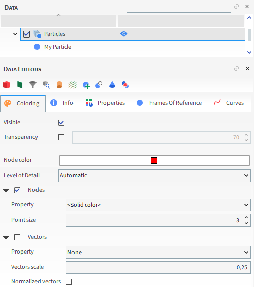
The Coloring tab, located on the Data Editors panel when a simulation entity is selected in the Data panel, helps you change the colors and data attributes of your selected entity.
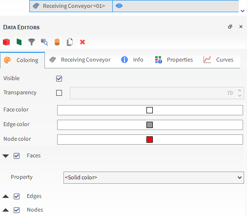
The options displayed on the tab are dependent upon which type of window you select. If a 3D Plot window is selected, the Coloring tab shows options that enable you to change the appearance of the entity you have selected in the Data panel (Figure 1). Those changes will be visible in the 3D View.
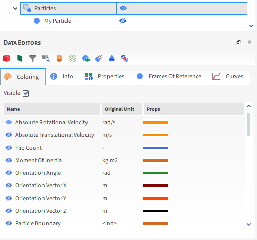
If a plot or histogram window is selected, the Coloring tab shows the data sets that are already calculated and ready to display in the window (Figure 2). The active data sets are indicated with an "open" eye icon. (See also Show/Hide Components by Using Eye Icons and Checkboxes.) Unlike when a 3D View window is selected, the data on the Coloring tab when a plot or histogram window is selected is not dependent upon what is selected in the Data panel.
If a Motion Preview window is selected, the Coloring tab shows options related to the axes of the Frame that is selected in the Data panel.
Figure 2.11: Coloring tab when a Motion Frame is selected in the Data panel AND a Motion Preview window is selected
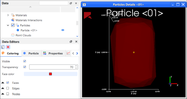
If a Particles Details window is selected, the Coloring tab shows options that will enable you to change the appearance of the particle shape you have selected to display. You can also adjust the transparency settings, allowing you to finely tune the opacity of the particle and achive the desired level of transparency (Figure 4).
See Also:
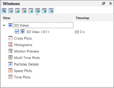
The Windows panel enables you to easily view, create, or remove the various Rocky windows-including 3D View windows, Motion Preview windows, and plots and histogram windows-all in one place (Figure 1).
It is hidden by default when you first open Rocky, but can be shown by selecting Windows from the View menu.
On the Windows panel, existing windows are listed below their categories, and new windows can be created from the button bar at the top of the panel. And by using the checkboxes, windows can be shown or hidden from the workspace without actually removing them from the project. (See also Show/Hide Components by Using Eye icons and Checkboxes.)
Selecting a window from this panel will enable that window's editable properties in the Window Editors panel.
See Also:
The Window Editors panel (Figure 1) displays the editable settings and parameters for the Rocky window that is selected in the Windows panel (see also About the Windows Panel).

Depending upon the type of window that is selected, different options will be presented, such as the following:
Window-type-specific options, such as background color, and font sizes.
Coloring, which provides options for displaying the data (geometries, graph lines, etc.) shown in the selected window.
Overlays, which provides options for adding text or images to the 3D View window.
Export, which provides options for exporting and then viewing images or data from the window outside of Rocky.
See Also:
The Log panel is for more advanced users of Rocky. Its purpose is to display the actions you have taken in the program that Rocky records for bug reporting purposes (Figure 1). When an error is shown in the program, you are sometimes given the option of submitting a report with your feedback. That report would contain details regarding the actions displayed in this panel.
This kind of information can be useful when writing and testing scripts. (See also About Creating and Using PrePost Scripts.)
For example, the actions displayed on the Log panel can be referenced while playing a script (Figure 1), which can be useful for debugging purposes.
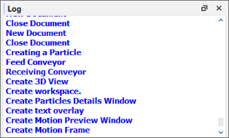 Figure 1: Log panel showing some actions that were recorded
In addition, if a print function is referenced when creating a script (Figure 2), it will appear in the Log panel when the script is played (Figure 3).
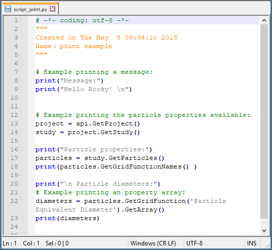 Figure 2: Example script making use of a print function
 Figure 3: Log panel showing print function when example script is played
The Log is for display only and cannot be edited. Like the Undo/Redo history panel (see also About the Undo/Redo History Panel), the items displayed in this panel are cleared every time you close and open the project.
See Also:
The Simulation Log panel displays any solver-related warnings, errors, or other information that happen during processing (Figure 1), no matter whether you are running your simulations using CPU or GPU resources. This kind of information can be useful when troubleshooting issues that occur when you process your simulation project.
Figure 2.15: Simulation Log panel showing some warnings and information that was logged during processing
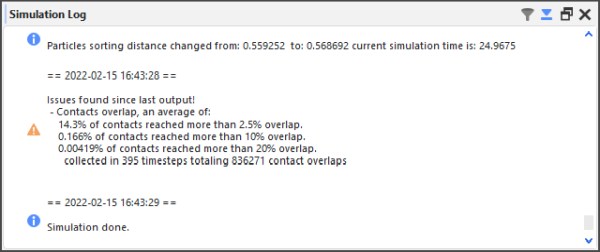
The Simulation Log is for display only and cannot be edited. But because it is possible to get many messages per simulation, you are able to filter the results and/or have Rocky automatically scroll to the bottom of the list by using the Filter and Auto Scroll buttons, respectively, at the top of the panel.
Unlike the other Log panels in Rocky, the items displayed in this panel are retained when the project is closed. This is to help you troubleshoot any issues with the Solver that might have caused Rocky to stop processing. It can also be useful in cases where you have used the Rocky Scheduler (see also About Processing Multiple Simulations In Succession) to process a project and want to review what errors or warnings were recorded by the solver during processing.
The Simulation Log is cleared whenever a new simulation or project is started.
Tip: For details about some of the more asked-about warnings and errors that can appear on your Simulation Log panel, see also I get warnings or errors on my Simulation Log Panel.
See the table below for information about the Simulation Log panel functionality.
Table 1: Simulation Log panel functionality
Button | Description | Range |
|---|---|---|
| Enables you to reduce the information shown to only messages of certain types. Messages are filtered by level of importance. Specifically:
Tip: To see all messages of any type, ensure that the Filter is set to Information. | Information; Warning; Error |
| Enables you to determine whether Rocky will automatically scroll the view area in the panel when new information is added, or will keep the view area stationary. Tip: To always see the latest messages without having to scroll down in the panel, ensure Auto Scroll is turned on. | Turns on or off |


See Also:
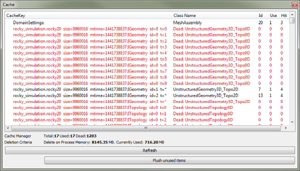
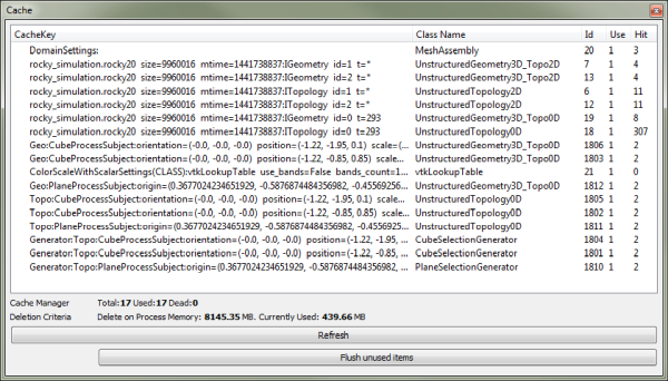
The Cache panel is for more advanced users of Rocky. It is designed to list the Rocky processes that take up memory (Figure 1), and also enables you to remove any unused processes that are no longer needed (Figure 2). This information can be used to optimize how Rocky uses the memory available.
Note: Memory allotment for Rocky is set from the Preferences dialog. (See also About Setting Global Preferences.)
Use the table below and images above to help you understand more about the Cache panel.
Table 1: Cache panel settings
Setting | Description |
|---|---|
Cache list | Lists individual Rocky processes taking up memory. Tip: Click the Refresh button to view the current list. |
Cache Manager | Counts the processes in the Cache list and organizes them by the following criteria:
|
Deletion Criteria | Describes how processes will be deleted. Specifically:
|
See Also:
The Debug Info panel is for advanced users of Rocky. It is designed to list code-related items for the purpose of solving issues found within the program (Figure 1).

See Also:
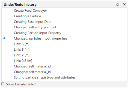
The Undo/Redo history panel Figure 2.19: Undo/Redo history panel showing some example actions is one way you can review and undo the actions you took on your project. Each separate step you take or setting you change is chronologically listed in this panel. When you Undo or Redo an action- either by using the panel, the toolbar, or keyboard - the choices you make are reflected here. The last action applied to the project is marked with a blue arrow; active actions are listed in black; inactive (or "undone") actions are listed in gray Figure 2.20: Undo/Redo history panel showing some example actions that have been undone.
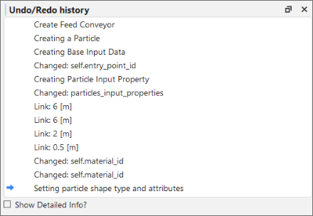
You can use the toolbar or keyboard to undo or redo one action at a time. You can use the panel to undo or redo every action up to the action you select. In this way, you can "undo" or "redo" as many actions as you like with only a double-click.
The actions listed in the panel are cleared every time you close and open the project.
What do you want to do?
Ensure the Undo/Redo history panel is open. (From the View menu, click Undo/Redo history.)
Do one of the following:
To undo several actions at once, find the blue arrow marking the current action, scroll up the list and then double-click the black-colored action to which you want to revert. The blue arrow now marks the action you selected and all later actions are colored gray to indicate that they are now inactive.
To redo several actions at once, find the blue arrow marking the current action, scroll down the list and then double-click the gray-colored action to which you want to redo. The blue arrow now marks the action you selected and all previous actions are colored black to indicate that they are now active.
See Also:
Do one of the following:
Click the Undo or Redo buttons on the toolbar.
Press Ctrl+Z or Ctrl+Y on your keyboard.
See Also:
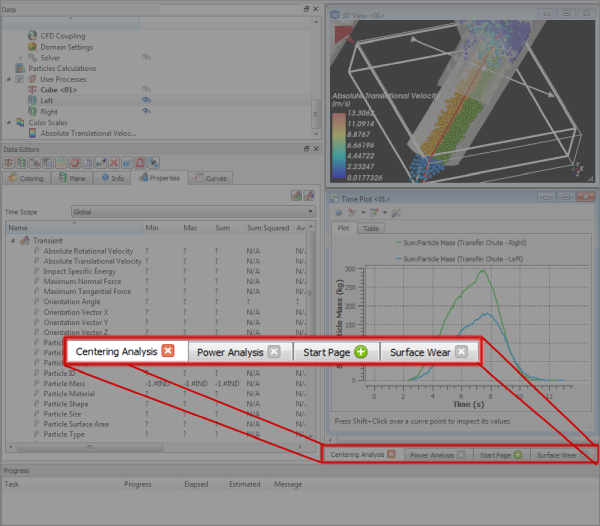
A Workspace is a collection of Rocky windows. Located in the center of the Rocky screen, the windows that make up a Workspace are where you choose to view the physical components of your simulation setup (3D View windows), and interact with the graphical results of your simulation (plot and histogram windows).
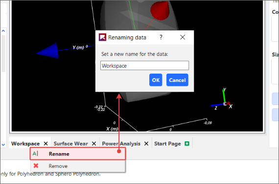
You can have multiple Workspaces for different purposes, such as by analysis type. These are designated by Workspace tabs along the bottom of the Workspace area Figure 2.21: Example tabs at the bottom of the Workspace area, which can also be renamed to help you better categorize your data Figure 2.22: Renaming a Workspace. You can also use the tiling options in the Windows menu to better organize your windows on the Workspace Figure 2.22: Renaming a Workspace.
What would you like to do?
See Also:
From the bottom of the center Workspace area, on the Start Page tab, click the green "+" icon. A new tab appears at the bottom of the Workspace.
Tips:
To change the name of the Workspace, right-click the Workspace tab and then in the Renaming data dialog, enter a new name and then click OK.
To add windows to the Workspace, see the following topics:
See Also:
Do one or more of the following:
To remove an existing Workspace, right-click tab for the Workspace you want to remove, and click the red "X" icon. Note: Removing the Workspace also removes any window(s) that you had placed on the Workspace. This can be reversed with the Undo function. (See also Undo or Redo a Single Action at Once.)
To add another Workspace, on the Start Page Workspace tab, click the green "+" icon.
To change the name of the Workspace, do the following:
Right-click the Workspace tab, and click Rename.
From the Renaming data dialog, enter a new name for the Workspace, and then click OK.
To arrange the windows orderly on a Workspace, from the Windows menu, select the Tile Columns option you want.
To add windows to the Workspace, see the following topics:
See Also:
This section covers the not-so-obvious but useful features scattered throughout the Rocky UI and how it might benefit you to use them.
What would you like to do?
See Input/Output Relationships in the Data Panel When Component Names are Bold
Determine the Frequency of Calculations by Pinning/Unpinning Items
Double-Click the Status Panel to Jump to the Appropriate UI Location
Refer to the Rocky Title Bar for Simulation Progress Details
Lock a Curve Selection to a Plot to Quickly Change the Data Shown
Double-Click a Plot Line, Bar, or Point to Change Its Appearance
See Also:
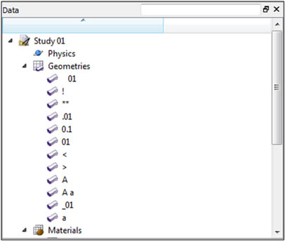
Sorting in Rocky follows the rules for Extended ASCII character codes (For a full list, see Appendix B: ASCII Printable Characters.) In general, Names beginning with spaces are sorted first, followed by most special characters, followed by numbers, followed by uppercase letters, and ending with lowercase letters.
For example, Rocky would sort the following 12 geometry components in the order shown in Figure 1.
See Also:
Rocky provides two complementary methods for determining whether a component or family of components will be shown or hidden in the Workspace: The eye icon (Figure 1), which affects the visibility of only that individual component, and the checkbox (Figure 2), which affects the visibility of all sub-components beneath the object.
![]() Figure 1 : Open and closed eye icons to the right of objects in the Data
panel
Figure 1 : Open and closed eye icons to the right of objects in the Data
panel
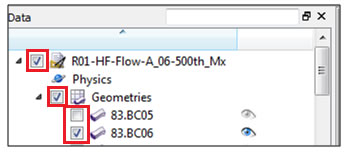 Figure 2 : Checkboxes to the left of objects in the Data panel
Eye Icon
An "open" eye icon (default setting) indicates that particular object is visible or shown in 3D View windows, plots, or histograms. A "closed" eye icon keeps that item in the simulation's calculations but makes the object appear invisible or hidden in the window. This is useful for seeing behind one object to another in an animation, for example, or for focusing on a particular curve in a plot.
Checkbox
In the Data panel, the checkbox has the same visibility affect as the eye icon but is hierarchical, meaning it affects all children components directly beneath that item in the Data panel. For example, clearing the checkbox to the left of Geometries hides all individual geometry components listed beneath it.
In the Windows panel, the checkbox acts like the eye icon does in the Data panel: it shows/hides the individual object—in this case, various windows in the Workspace. Unlike in the Data panel, checkboxes in the Windows panel are not hierarchical.
See Also:
Linked objects refer to the ability of a geometry component, Particles, or 1-Way LBM to provide data to a particular User Process, thus establishing an input/output relationship between them. This linkage is illustrated in the Data panel by the name of the object providing the data (output) turning bold when the User Process that is accepting the data (input) is selected, as shown in Figure 1.
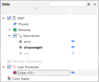 Figure 1 : Example of a geometry component shown in bold when the user
process linked to it is selected
Figure 1 : Example of a geometry component shown in bold when the user
process linked to it is selected
To create this kind of input/output relationship, the User Process must be created directly from the object providing the data. In the example above, the Cube <01> user process was created by selecting the dropweight geometry and then creating a Cube user process from either the Data Editor or right-click menu.
See Also:
After processing your simulation, you can view various types of data on the Properties and Curves tabs for your simulation settings like particles and geometry components. Each of the items listed on these tabs has a pin icon to the left of it, as illustrated in Figure 1.
![]() Figure 1 : Pin icons on the Properties tab of the Data Editors panel
Figure 1 : Pin icons on the Properties tab of the Data Editors panel
The color of these pin icons indicates how often Rocky calculates the particular item, as follows
A gray-colored pin (default) indicates that the item will not be calculated for any output time. Choosing to avoid calculating data that you don't need saves processing time and power during your simulation
A red-colored pin indicates that the item will be calculated for each output time included in the simulation. And if settings affecting those values change, Rocky will recalculate to keep all the values current. Important: Choosing to have Rocky calculate the item at each output time is likely to take up a significant amount of processing time and power. Only choose to pin items for which having all output time calculations be kept up-to-date and available are truly necessary for your analysis.
Tip: To pin or unpin an item, just left-click the pin icon.
Alternately, you can choose to have Rocky calculate any values you are interested in once, by right-clicking the item and choosing Compute Statistics. (See also About Viewing an Individual Statistic.)
See Also:
Rocky uses several different characters and strings as placeholders for calculations or explanations that would take up too much room in the UI. Here is a quick list of some placeholders you might run across and what they mean.
Note: These placeholders might appear on the Info, Properties, or Curves tabs (Data Editors panel).
Placeholder | Description |
|---|---|
? | Information isn't calculated yet. Same as "Not loaded." |
Not loaded | Information isn't calculated yet. Same as "?". |
- | Item contains no unit for the value displayed. Generally indicates a ratio, such as a percentage. |
Unable to calculate | Not enough information available at this particular output time in order to calculate the values. |
Unknown | Not enough information is known to calculate the value. |
<ind> | Item contains no units for the value displayed. Generally indicates a index, such as a count or a coordinate position. |
-1.#IND | Calculation is invalid. This can happen to Particle properties, for example, if there are no particles in the simulation at the time specified for the calculation. |
N/A | Value is Not Applicable (N/A) to the selected item. |
See Also:
If you have errors listed in the Status panel (Figure 1), you can double-click those errors to be taken to the location in the Data panel where you would address them.
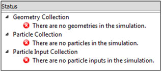
For example, if you double-click the "There are no geometries in the simulation" error, Rocky would enable the Geometries item in the Data panel.
See Also:
Rocky provides instant feedback for entering functions and variables into a parameter text field by coloring the text as you type, as explained below:
Red text indicates that the syntax of the active entry is not yet valid. The syntax is based upon the rules of the Python programming language. It will tell you whether you have an open parenthesis that needs to be closed, for example.
Green text indicates that the syntax of the active entry is valid. Note: Green text does not indicate that the value, function, or variable of active entry has been formatted correctly or is itself a valid entry. Validation happens after either pressing Enter or clicking away from the text field.
Black text indicates a currently inactive entry.
See Also:
There are several tasks in Rocky that can be accomplished more easily by dragging items with your mouse and dropping them to another location, as described below:
Creating new views of Particles, individual geometry components, or Air Flow: From the Data panel, select the component(s) you want to view and then drag and drop them to a window of your choice (3D View, Histogram, or Time Plot). Only the component(s) you selected will be added.
Creating new views of data sets: From the Data Editors panel, on the Curve or Properties tab, select the data item(s) you want to show and then drag and drop them into the window type you want (3D View, plots or histograms).
Creating multiple Multi-Time plots in a single window: After adding your first data set, hold the Ctrl key while selecting your next data set and then drag and drop it into the gray area of an existing Multi-Time plot window. Another plot appears in the same window.
Tip: You can also multi-select items to drag and drop. (For example, show multiple geometry components at once in a 3D View.) Just hold the Ctrl or Shift key while left clicking your selections with the mouse, and then drag and drop as usual.
See Also:
There are a few things in Rocky that can only be accomplished by right-clicking the item, as described below:
Adding/Importing geometry components: From the Data panel, right-click Geometries to access the menu that enables you to add or import new geometry components.
Computing statistics for only the current output time: From the Data Editors panel, on the Curves or Properties tab, right-click the data item you want to view values for and then click Compute Statistics from the right-click menu.
Showing only a few components in a new window: From the Data panel, select the item(s) you want displayed in a new window, right-click your selection, and then from the right-click menu, point to Show in New and then click the window type you want. Only the items you selected appear in the new window.
Import your own User Process shape for particle analysis: From the Data panel, right-click Particles, point to User Processes, and then click Polyhedron (Envelope). From the Select the STL file for the polyhedron dialog, navigate to the STL file you want, and then click Open. The polyhedron you chose appears under the User Processes list. Note: You can also create a custom-shaped User Process from any existing User Process that was originally created from a Particle set. (See also See Input/Output Relationships in the Data Panel When Component Names are Bold.) From the Data panel, under User Process, right-click a User Process that was created from a Particle set and then follow the instructions above.
See Also:
The search bar is located at the very top right of the Data panel, as shown in Figure 1.
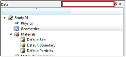 Figure 1 : Data panel search bar
When you start typing into it, Rocky immediately displays in the Data panel the entire hierarchy of the component(s) that best match what you typed. In a simulation setup with many different components, using the search bar can help you find what you need faster than scrolling.
Tips:
To search the names in order from left to right, enter the first few characters of the component you want to find. For example, to find all components that begin with "belt," type belt into the search box. You would find "belt 01" and "belt 02" but not "feeder belt" by using this method.
To search anywhere in the name, type an asterisk (*) followed by the characters anywhere within the name that you want to find. For example, to find all components containing "belt" anywhere in the name, type *belt into the search box. In this way, you would find the "feeder belt" component as well as "belt 01" and "belt 02."
See Also:
When you are actively processing a simulation (see also About Starting a Simulation), the Title bar for the Rocky program displays useful details about the simulation's progress. (Figure 1.)
 Figure 1 : Example of Title bar progress information shown while a
simulation is processing
Figure 1 : Example of Title bar progress information shown while a
simulation is processing
This progress information in the Title bar includes the following:
Output: The total number of output files that have been saved thus far. In the example in Figure 1, the total number of output files saved so far is 81.
Current progress: The particular second of the total Simulation Duration that Rocky is currently calculating. Note that Rocky calculates in finer detail than is typically determined by the Output Frequency in which it saves output files. In the example in Figure 1, although Rocky is currently calculating for second 4.050, because the simulation output frequency is set to 0.05 seconds, it won't actually save a 82nd output file representing 4.100 seconds until the current progress reaches that point.
Elapsed: Amount of real time since starting (or resuming) the simulation processing. In the example in Figure 1, 12 seconds have elapsed since the simulation was resumed.
ETA: Rocky's estimate of how much real time the simulation will take to complete. This is a rough approximation Rocky extrapolates based upon the amount of time the last several outputs took to calculate. In the example in Figure 1, Rocky estimates that it will take roughly 2 minutes and 49 seconds to complete. The ETA will get longer as more and more particles enter the simulation and it takes more time for Rocky to calculate each output. Should the simulation reach a point where more particles leave the simulation than enter it, the ETA will begin to get shorter. Once the simulation enters a steady state, this value will likely be a very good estimate of the remaining time.
See Also:
If you want to see the same curve (for example, Particle Mass) in a plot (for example, Time Plot) across many similar Data panel elements (for example, several User Processes created from Particles), you can use the Replace Curves According to Data Tree Selection toggle button (Figure 1), which is available for any Time Plot, Multi Time Plot, or Cross Plot.
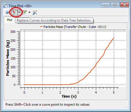
When you toggle (push in) this button on a plot you have created and then select another similar item on the Data panel, the curve you original selected stays the same but the data is replaced with the data corresponding to the item you just selected (Figure 2).
Figure 2.27: Original plot (top); second Data panel option selected with button toggled (middle); third Data panel option selected with button toggled (bottom)
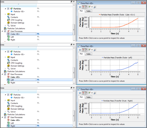
In this way, you can quickly compare the same curve across many similar Data panel items without having to create many separate plots. This button also works if you multi-select curves.
To turn off this feature, click the toggle button again to push it out.
See Also:
Similar to the Edit Expression dialog that you get when you click the Edit Formula button on the Table tab of a Time Plot (see also About Time Plots), you can also change the Pen style, color, and width as well as the data point appearance by double-clicking the line, bar, or point in the plot or histogram. This will bring up the Edit Curves dialog (Figure 1) and from there, you can change the settings as you like.
Tip: You can also right-click the line, bar, or point and then from the menu, select the Edit option pertaining to the curve you want to change. This will bring up the same Edit Curves dialog you get when you double-left-click (Figure 1).
See the image, table, and procedure below for information about the Edit Curves dialog.

Table 1: Edit Curves dialog options
Setting | Description | Range |
|---|---|---|
Curves | Enables you to select which data set(s) you want to change. | Options limited by the plot or histogram selected |
Pen | ||
Style | For plots only (not histograms), this enables you to set what kind of line style you want represented for the selected data set. Tip: If you want the data set represented on the plot by symbols instead of lines, select No Line and then choose what you want under Symbol. | No Line; Solid Line; Dash Line; Dot Line; Dash Dot Line; Dash Dot Dot Line |
Curve Style | For plots only (not histograms), when you select a Style other than No Line, this enables you to set how the data set is represented in the plot. What you set here will be drawn in the Style indicated. | Lines; Sticks; Steps |
Color | For histograms, and also for plots with a Style other than No Line, this enables you to change the color of the bar or plot line for the selected data set. | Options limited by the Select Color dialog |
Width | For plots only (not histograms), when you select a Style other than No Line, this enables you to change the width of the plot line for the selected data set. | Whole numbers greater than or equal to one |
Symbol | ||
Shape | For plots only (not histograms), this enables you to add to the plot a symbol marking the curve's data point. For Time Plots and Multi Time Plots, a symbol will appear for each recorded output time. (For example, every 0.05s.) Tip: If you want the data set represented on the plot by lines instead of symbols, select No Symbol and then choose what you want under Pen. | Ellipse; Rectangle; Diamond; Triangle; Down Triangle; No Symbol |
Color | For plots only (not histograms), when you select a Shape other than No Symbol, this enables you to change the color of the symbol used to mark the data points of the curve. | Options limited by the Select Color dialog |
Size | For plots only (not histograms), when you select a Shape other than No Symbol, this enables you to change the size of the symbol used to mark the data points of the curve. | Whole, positive values |
Directly within the plot or histogram window, double-click the line, bar, or point that you want to change. The Edit Curves dialog appears.
From the Curves box, select the data set(s) you want to modify.
Under Pen and Symbol, select the options you want.
Click OK. The changes you made are reflected in the plot or histogram window.
See Also:
Occasionally, Module parameters in Rocky will be shared by parameters of other Modules. This means that a value entered in one location in the Rocky UI will be automatically duplicated in the other location.
To help you understand when this is happening, Rocky will place an asterisk (*) after the parameter name that is being shared. If you then hover your mouse cursor over the field for that asterisked parameter (Figure 1), the tooltip that appears will tell you what other Modules are sharing that same parameter.
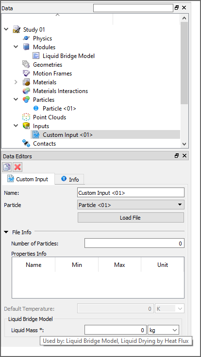
In the example shown in Figure 1, the asterisk following the name of the Liquid Mass* parameter indicates that there are one or more identical Liquid Mass parameter(s) being defined elsewhere in the Rocky UI. When you view the tooltip for this parameter's field, you learn that this parameter is shared by two separate Modules, this one included.
If you change the value for this shared parameter, it will automatically be updated in the other location(s).
Note: In this version of Rocky, the Liquid Bridge Model Module is provided as an external module. Refer to the Install an External Module topic for details.
See Also:
When viewed in a 3D View window, you can change the shape and location of some User Process, Volume Fill, and Region of Interest shapes by using the colored directional handles, as shown in Figures 1 and 2 below.
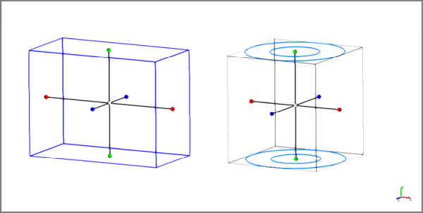

For shapes like Cubes and Cylinders (Figure 1), the colors of the handles are defined in Table 1.
Table 1: Handle color definitions for shapes
Handle (Dot) Color | Corresponds To |
|---|---|
Red | The local X axis. |
Green | The local Y axis. |
Blue | The local Z axis. |
White | The center of the shape. Note: For Volume Fill shapes, the blue dot in the center is the Seed location but this can only be moved by defining the Seed Coordinates. (See also Create a New Volume Fill Input for Particles.) |
For planes (Figure 2), the directional handles are colored according to the Font Color specified for the 3D View (see also About Using the Window Editors panel to Change the Selected 3D View). The shapes of these colored handles are defined in Table 2.
Table 2: Handle shape definitions for planes
Handle Shape | Corresponds To |
|---|---|
Dot | The location of the plane's origin. |
Arrow | The direction of the plane's normal. |
Within the 3D View window, you can click and drag these handles to the new location you want.
Tip: To move the whole shape without deforming it, do one of the following:
Move only the center handle.
Hold either the Shift or Ctrl key while you click and drag any of the outer handles with your mouse.
Or, for more precise control, you can enter exact values in the Data Editors panel.
See Also:
While Rocky was not designed for full software accessibility, it does offer some limited features for keyboard control. For example:
TAB key: Press to move from option to option within a Rocky dialog or panel.
SPACEBAR: Press to select or clear a check box, or to select buttons in panels.
UP/DOWN ARROW keys: Press to select list items within a Rocky dialog, Panel, or menu.
LEFT/RIGHT ARROW keys: Press to view different menus or to move horizontally in Rocky dialogs.
ESC key: Press to close a dialog.
ENTER: Press to select a button within Rocky dialogs.
From the Options menu, click Preferences.
From the Preferences dialog, under Properties, click Shortcuts.
See Also:
There are several unique file types and folders used in Rocky, and several common ones. Use the tables below to identify when and why certain file types and/or folder locations are used.
Note: Only the simulation project file is saved to the directory location you choose. All other files created by Rocky (marked as "System" below) are saved to a project subfolder created automatically within the same directory as your project file. System files are critical for Rocky functioning and should not be edited, moved, or deleted.
Files you choose to export out of Rocky, including animation, image, and data files, are saved to the locations you specify. See the below tables for more detail.
Table 1: File Types Used in Rocky
Type | Description | Extension |
|---|---|---|
Rocky Simulation Files | ||
Simulation project file (Rocky v4 or later) | Contains all parameters set and analyses completed for a particular simulation created in Rocky 4 or later, and is linked to the simulation output files (.rhs, .rhc, and .rhm) that are created during processing.
| .rocky |
Simulation project file (Rocky v3 only) | Contains all parameters set and analyses completed for a particular simulation created in Rocky 3, and is linked to the simulation output files (.rhs) that are created during processing. Tip: Use the extension of the simulation project file to help you determine in which version of Rocky the project was created. Projects created in older versions of Rocky will have different features than those created in Rocky v4 or later versions. | .rocky30 |
(System) Simulation output file for particles and boundaries | The particle- and boundary-related results of the simulation that are created during processing. One output file is saved per simulation output frequency; many output files make up a whole simulation.
| .rhs |
(System) Simulation output file for contacts | The contact-related results of the simulation that are created during processing. This data is required to calculate particle and boundary movement and is by default saved for each output time to help make Resuming a Stopped Simulation faster. (See also Resume Processing a Stopped Simulation.) Tip: To reduce the size of your project files, clear the Collect Contacts Data ** checkbox. (From the **Data panel, click Contacts and then from the Data Editors ** select the **Contacts tab.) (See also About Contacts.) | .rhc |
(System) Simulation output file for motions | The motion-related results of the simulation that are created during processing. One output file is saved per simulation output frequency; many output files make up a whole simulation.
| .rhm |
(System) Solver file | Used for storing information related only to the setup and calculated results of the simulation. Does not include post-processing information, such as views, graphs, or animations. | .rocky20 |
(System) Solver output files | System files containing runtime simulation information meant to be processed by the application. (See also About the Simulation Log File.) | .rocky20.log .rocky20.out .rocky20.prg |
Rocky lock file | System file used to prevent another instance of the currently active project from being modified elsewhere. This file is created automatically by Rocky every time you open a project and remains on your system until you close the project, essentially locking the project file from being changed by anyone but you as long as you have the project open. This feature is especially useful in shared computing and server environments where multiple users may be contributing to the same Rocky projects but using different computing resources. It is for this reason that modifying, moving, or deleting the lock file is not recommended unless you are certain no other copies of the project are being worked on. (See also Rocky says my project file is "locked".) | .lock |
(System) Current output file | This is where Rocky saves the initial and final output time value, which is used to determine the current output time. | _H.txt |
Rocky script file | File used to contain script information, the latter of which includes recorded steps of a repeatable UI task. (See Creating and Using Your Scripts for more information.) | .py |
Rocky archive file | File used to contain all simulation project and supporting folders necessary for sharing the simulation project and results with others, such as Rocky support. (See also Archive a Simulation Project.) | .rocky_archive |
Rocky project context file | File used to contain the setup criteria for the 3D View windows, Workspaces, and User Processes used in the project. (See also Reuse 3D View Window, Workspace, and User Process Setups in Other Projects. | .rocky_template |
Files Exported Out of Rocky | ||
Simulation statistics file | File created by exporting curves from a plot or histogram, thereby enabling the data to be viewed and/or edited in an external spreadsheet program, such as Microsoft Excel. | .csv |
Animation file | File created by exporting an animation, thereby enabling the simulation to be viewed outside of Rocky. (See About Creating and Saving an Animation for more information.) | .avi |
Image files | Used for saving or exporting a snapshot of what is currently being displayed in a window on the Workspace, or for importing into Rocky as a logo to be shown in the 3D View. | .png .jpg .bmp .pnp |
Files Imported Into Rocky | ||
3D CAD model files | Used for importing geometries into Rocky.
Note: Unlike in previous versions, none of these file types retain the component colors assigned in the CAD model upon import into Rocky. | .xgl .stl .dxf .msh |
Fluent Case file | Used for importing geometries from an Ansys Fluent case file into Rocky. Geometry component names will be retained in this scenario. Also used to specify the Ansys Fluent simulation setup for 2-Way Fluent Coupling analyses. Contains the grid, boundary conditions, solution parameters and other data related to a fluid flow simulation problem. | .cas |
Fluent Case file (compressed) | Compressed version of a Fluent Case file (CAS). Used both for importing geometries from an Ansys Fluent case file into Rocky, and also to specify the Ansys Fluent simulation setup for 2-Way Fluent Coupling analyses. | .cas.gz |
Fluent Case file (HDF5) | Hierarchical Data Format (HDF) version of a Fluent Case file (CAS). In this version of Rocky, CAS.H5 files can be used both for importing geometries, and to specify the Ansys Fluent simulation setup for 2-Way Fluent Coupling analyses. | .cas.h5 |
Fluent Mesh file | Used for importing geometries from Ansys Fluent into Rocky. Geometry component names will not be retained when importing a MSH file into Rocky. | .msh |
Ansys Motion Functional Mock-Up Unit file | Bundled file containing all motion setup information required for a 2-Way Coupled simulation with Ansys Motion, including geometries. As such, can be used for geometry import into Rocky. Currently supports only rigid bodies (no flexible bodies) without beam elements. (For more information about beam elements, refer to your Ansys Motion documentation.) Geometry component names will be retained with this type of file import. Important: Only FMU files generated by Ansys Motion will support geometry import into Rocky. | .fmu |
Ansys Motion Geometry file | Used for importing geometries from an Ansys Motion file into Rocky. Currently supports only rigid bodies (no flexible bodies) without edge elements. Geometry component names will be retained with this type of file import. | .dfg |
Fluent to Rocky file | File generated by the Fluent plug-in installed by Rocky. Used for importing fluid flow data out of Ansys Fluent and into Rocky. Depending upon the export type chosen, produces either a static or transient fluid flow model within the simulation. (See About Using the 1-Way Fluent Method for more information.) | .f2r |
Fluent Data file | File containing Fluent initialization settings and the values of the specified flow field that can be used during a 1-Way Fluent or 2-Way Fluent coupling simulation. (See also About Using the 1-Way Fluent Method and About Using the 2-Way Fluent Method.) | .dat |
Fluent Mesh Data file | File containing CFD mesh location data that can be used in a 1-Way Fluent coupling simulation. (See also About Using the 2-Way Fluent Method.) | mesh.dat |
Fluent Data file (Compressed) | Compressed version of a Fluent Data file (DAT), which is an optional file containing Fluent initialization settings that are used during a 2-Way Fluent coupling simulation. (See also About Using the 2-Way Fluent Method.) | .dat.gz |
Fluent Data file (HDF5) | Hierarchical Data Format (HDF) version of a Fluent data file (DAT), which is an optional file containing Fluent initialization settings that are used during a 2-Way Fluent coupling simulation. (See also About Using the 2-Way Fluent Method.) | .dat.h5 |
Custom Fiber definition file | Text or spreadsheet file used to define the Segment details that make up a Custom Fiber shape. (See also About Defining and Importing Custom Particle Shapes.) | .txt .csv .xls .xlsx .xlsm .xlsb .odf |
Custom Input definition file | Spreadsheet file used to define the particle positioning details that make up a Custom Input. (See also About Adding and Editing Particle Inputs.) | .csv .xls .xlsx .xlsm .xlsb .odf |
Point Cloud definition file | Text file used to define the details that make up a Point Cloud. (See also About Point Clouds.) | .txt |
Table 2: Common Folder Locations Used in Rocky
Folder | Typical Windows Location | Typical Linux Location | Description |
|---|---|---|---|
Rocky Settings |
|
| Folder where Rocky stores settings that persist from project to project. These include license settings, a list a list of recently opened projects, and a separate "Settings" folder that contains your display and interaction preferences. (See below.) |
Rocky Preferences |
|
| Folder where Rocky saves user preferences for various display and interaction settings. These settings can be established by users in the Preferences dialog (see also About Setting Global Preferences), or in several other Rocky locations by clicking a Save Current Configuration in Settings button. Both the values displayed on the Preferences dialog and the ones displayed on the UI element after the Restore Configuration from Settings button is clicked reflects the values saved to this folder. |
User Manual Cache |
|
| Contains the cache for the user manual. |
Shared PrePost Scripts |
|
| Folder where Rocky saves scripts you recorded on the Scripts shared across projects tab of the PrePost Script panel. Also where you save PY script files that have been created outside of Rocky using the API:PrePost functionality. (See also Creating and Using Your Scripts.) |
Project-Only PrePost Scripts |
|
| Folder where Rocky saves scripts you recorded on the Project scripts tab of the PrePost Script panel. Also where you save PY script files that have been created outside of Rocky using the API:PrePost functionality. (See also Creating and Using Your Scripts.) |
External Modules |
|
| Folder where you save the compiled external Module that you either create yourself or download from the Customer Portal. (See also About Rocky Modules and API:Solver - Functional Modules Page |
Tip: Performing a clean install of Rocky may involve renaming and/or archiving these folders after uninstalling Rocky and prior to reinstalling it. (See also I reinstalled Rocky but I am still seeing errors.)
See Also:
The simulation log is one of the solver output files that Rocky provides while processing a project. (See also File Types and Folders in Rocky). It contains simple information, such as hardware details, to more complex data about the simulation, such as particles, triangles, and contacts information; memory consumption and free memory; and other solver process information.
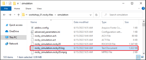
To access the simulation log file for a specific project, follow the steps below:
Navigate to the folder containing the project for which you want to see simulation details.
Open the project_name.rocky.files folder.
Open the simulation folder.
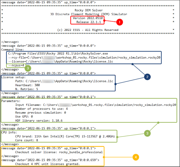
The simulation log file is located inside the simulation folder and is named rocky_simulation.rocky20.log (as shown in Figure 1). It is a Text Document, so you can open it with any text editor.
Inside the file, information is arranged similarly to the figures shown in this section. Some key areas are enumerated and explained below.
In Figure 2 (shown below), you can see the following:
Product release and version used to process the Rocky project. (See also About This Version of Rocky.)
License file information
Hardware details
Used licenses. (See also Verify Your Rocky License Status.)
Next, you will see everything that is related to the project setup including the physical models enabled, particle groups defined, materials, boundary limits, solver options, coupling mode, motion frames, and more (Figure 3).

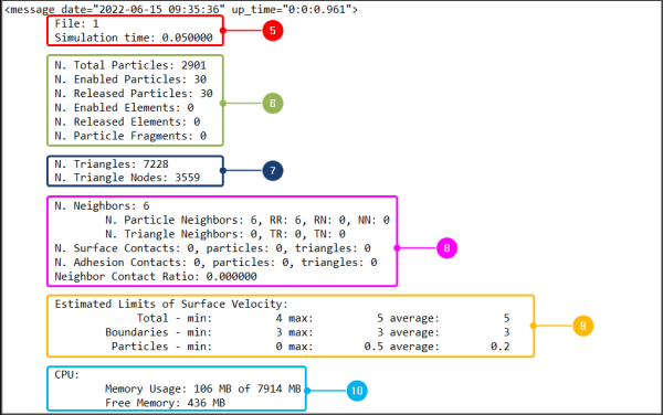
After that, the file shows a structure (Figures 4 and 5) that repeats for each output time and contains the following details:
File number (that refers to the output time) and simulation time
Particle and fragment counts. (See also About Particle Breakage.)
Triangle counts
Contact counts and ratios. (See also About Contacts.)
Limits of surface velocity
Memory (consumption and availability). (See also About the Cache Panel.)
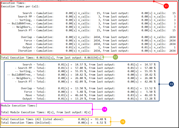
Average time per call and number of calls for each process. Note: Depending on the case, the processes will be different.
Execution times: both the total and since the last output
Total execution time, which is the average time per call multiplied by the number of calls
Execution times for the module: both the total and since the last output
Total execution times, which are the total measured and segregated times by the solver in the last output plus the fraction of time not measured by the solver
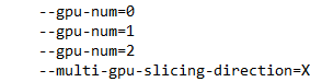
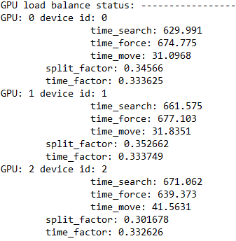
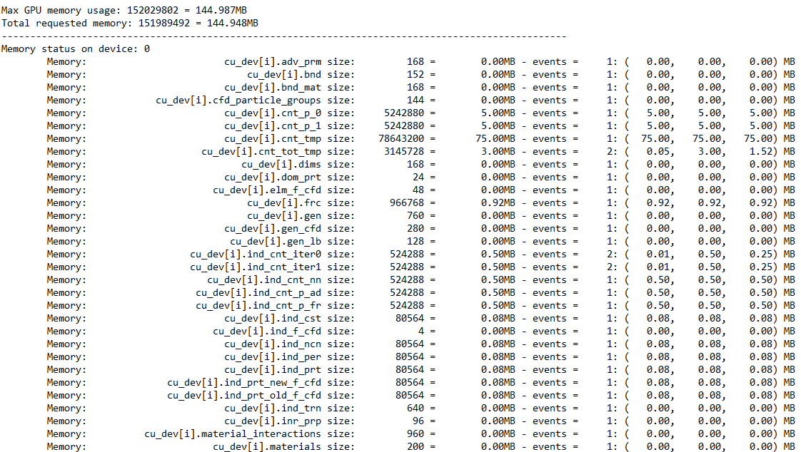
Finally, we have some additional information for simulations with GPU usage. Figures 6-8 show an example of a simulation log file for a project processed with 3 GPUs. The data shown includes the following:
GPUs IDs
GPU load balance with the time spent in each process and the split factor.
Tip: The slipt factor indicates the memory consumption of the GPU in relation to the total memory consumption (from all GPUs). In this example, as we have 3 GPUs, the ideal is to have a split factor close to 0.333.
Memory consumed in each device
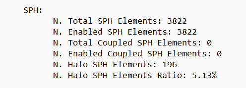
N. Halo SPH Elements/Halo Particles: In multi-GPU runs, halo particles/elements are those that are located in the overlapping devices domain regions and therefore are present simultaneously in two GPU devices. For the halo particles/elements, both devices compute the collision forces, but only one of the devices accumulates these data in order to perform velocity and displacement calculations.
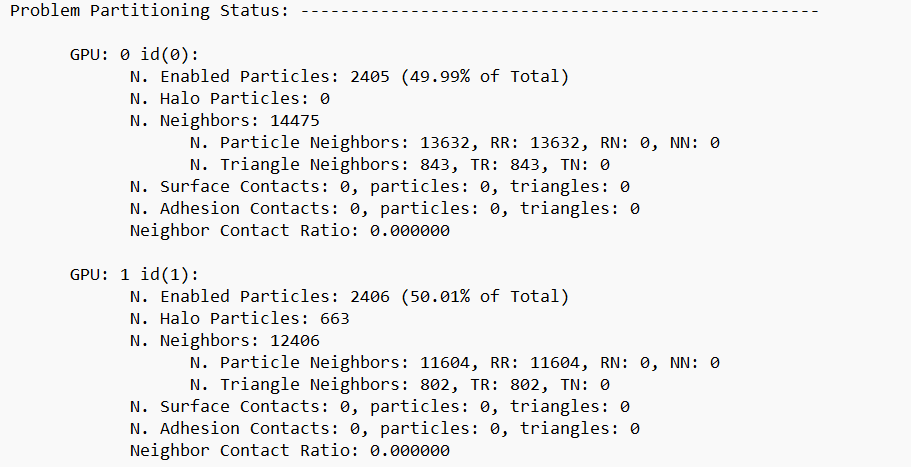
Problem Partitioning Status: This parameter represents the number of SPH Elements or particles coupled in the simulation.
N. Enabled Coupled SPH Elements: It is the number of SPH elements figured inside the particles for the purpose of interacting with external SPH elements in an SPH-DEM interaction simulation. This parameter will only be computed in simulations with SPH and DEM, otherwise it will appear as zero.
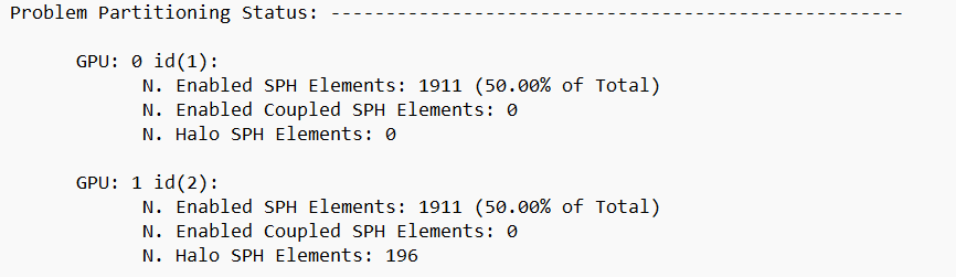
Note: If you processed your simulation without GPU usage, your simulation log file will not show this data. You can see how many GPUs were used by looking at the section marked "3" in Figure 1. (In that simulation example, "Use GPU: 0" means that the project was processed without GPU usage.)
In Rocky, some data is collected automatically and some data you must first opt in to collecting before you process your simulation. In addition, some data is always collected right from the start of the simulation, and some data waits to be collected until passing certain thresholds that you define.
Use the topics below to help you understand what, how, and when data is collected in Rocky.
Learn more About Collecting Data in Rocky
Learn more About Monitoring Overlaps
Learn more about Collecting Data on Boundaries
Learn more about Collecting Data on Particles
Learn more about Collecting Data on Contacts and Energy Spectra
See Also:
Rocky provides many options for calculating, collecting, and analyzing different kinds of data.
Since calculating data you do not want can slow down your processing, and retaining data you do not need can take up valuable storage space, Rocky requires you to opt-in (or turn on) certain kinds of data collection. It does this to help you maximize your computing power and storage space.
To help you better understand how and when data is calculated, use the table below and the topics that follow.
Table 1: Rocky data and statistics collection matrix
Type of Data or Statistic | How Collected | When Collected | See Also |
|---|---|---|---|
Affecting Geometries | |||
Surface wear modification | Opt-in via the Use Wear checkbox (located on the Geometry | Wear tab) prior to processing. | After Wear Start value is reached. | Enable and View Surface Wear Modification on an Imported Geometry |
Collision effects on belts and boundaries as a result of particles interactions | Opt-in via the Boundary Collisions Statistics Module prior to processing. | Immediately | Enable and View Collision Statistics for Boundaries |
Belt or boundary motions | Automatic collection | Immediately | About Curves |
All other data related to geometries | Automatic collection | Immediately | About Properties, About Curves |
Affecting Particles | |||
Particles energy spectra | Enable the Particles Energy Spectra module prior to processing. | After the module's Start Time value is reached. | Enable and View Data for Particles Energy Spectra |
Particle breakage | Automatic collection | After Breakage Start value is reached. | Enable and View Particle Breakage |
Fluid effects upon individual particles | Opt-in via the CFD Coupling Particle Statistics Module prior to processing. | After CFD Coupling Start Time value is reached | Enable and View Fluid-Related Statistics for Particles |
Collision effects upon the surface of a Particle set | Opt-in via the Intra-particle Collisions Statistics Module prior to processing. | Immediately | Enable and View Collision Statistics for Particle Surfaces (Intra) |
Collision effects upon each particle-particle and particle-boundary pair group within the simulation | Opt-in via the Inter-group Collision Statistics Module prior to processing. | Immediately | Enable and View Inter-group Collision Statistics for Particles |
Collision effects upon individual particles resulting from interactions with other particles and boundaries | Opt-in via the Inter-particle Collision Statistics Module prior to processing. | Immediately | Enable and View Collision Statistics for Particles Between Other Particles (Inter) |
Energy data for all Particle sets in the simulation | Opt-in via the Particle Instantaneous Energies Module prior to processing. | Immediately | Enable and View Instantaneous Energies for Particles |
All other data related to particles | Automatic collection | Immediately | About Properties, About Curves |
Affecting Contacts | |||
Contacts energy spectra | Enable the Contacts Energy Spectra module prior to processing. | After the module's Start Time value is reached. | Enable and View Data for Contacts Energy Spectra |
Stress-related data (for analyzing via Eulerian Statistics User Process) | Opt-in via the Collect Contacts Data checkbox on the Contacts entity prior to processing. | Immediately | Turn On Contacts Data Collection |
All other data related to Contacts | Opt-in via the Collect Contacts Data checkbox on the Contacts entity prior to processing. | Immediately | Turn On Contacts Data Collection, About Contacts |
Affecting all other Rocky entities | |||
All other data related to all other entities | Automatic collection | Immediately | About Properties, About Curves |
Note: If you have defined a Multiple Element (meshed) particle, what you have set for Meshed Particles Upscaling affects whether and how some post-processing properties and curves are displayed. (See also About Meshed Particles Upscaling.)
No matter how or when the data you want is collected, the resulting Properties (see also About Properties) can be visualized after processing in a view window and/or analyzed through a plot or histogram window. In addition, any resulting Curves (see also About Curves) can be analyzed through a plot or histogram window.
If you cannot see any of your simulation data and you know you have both collected it and have completed as much of the processing for which you want to have data, then you most likely have not yet created a view, plot, or histogram window by which to view and/or analyze the data or statistics you have collected.
Tip: Once your plot or histogram window is created (see also Graph Data within Rocky by Creating a Plot or Histogram), you can then modify the display to your liking (see also About Changing the Appearance of a Graph (Plot or Histogram)), export the data into a CSV file for further analysis outside of Rocky (see also Export Data into a CSV File), and more.
See Also:
In Rocky versions prior to 2022 R1, there was a built-in contact overlap monitor whose purpose was to check each contact pair (particle-particle or particle-boundary) for the amount that they overlapped, the percentage of which was determined by the size of the smallest particle in the contact pair.
During simulation processing, if at any timestep a contact pair's overlap exceeded one of three warning levels fixed at 2.5%, 10%, and 20%, a Contacts overlap message would be raised on the Simulation Log panel (Figure 1). (See also I get warnings or errors on my Simulation Log Panel.)
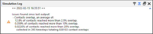
Monitoring your contacts for the size of their overlaps is important because Rocky is based on the soft-sphere approach, which uses the overlap value in order to compute collision forces. For example, in a typical simulation overlaps of 2.5% might be considered acceptable; however, simulations with overlaps larger than 10-20% should probably not be trusted as overlap values that large can lead to serious stability and accuracy issues.
Although it is a good practice to monitor overlap levels to guarantee they are below the desired values for a DEM solver, for some types of projects, the default warning levels Rocky uses might not be appropriate; or, it might be desired for there to be no overlap checks at all.
Therefore, as of Rocky 2022 R1, you are able to choose:
Whether or not you want contact overlaps to be monitored. Note: The monitor is "on" by default to match the behavior in older versions of Rocky.
What three overlap levels about which you want to be warned. Note: The initial values are set as to match the warning levels used in older versions of Rocky.
These tasks are accomplished via an embedded Module called Contacts Overlap Monitor (Figure 2).
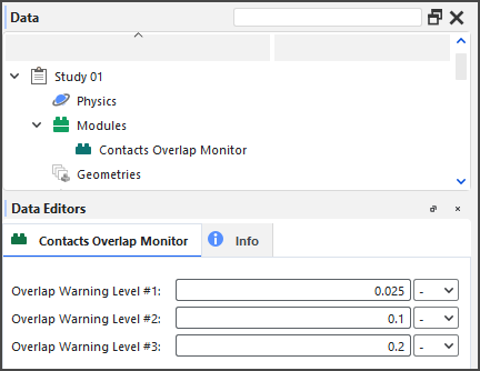 Figure 2: Options in the Data Editors panel for the Contacts Overlap Monitor Module
Use Figure 2 above and the table below to understand how to monitor your contact overlaps.
Table 1: Modules, Contacts Overlap Monitor parameter definitions
Setting | Description | Range |
|---|---|---|
Overlap Warning Level #1 | Defines the value of the first (of three) overlap warning thresholds. If a contact pair's overlap-the percentage of which is based upon the size of the smallest particle in the contact pair-exceeds this value, a message will be raised on the Simulation Log panel. (See also About the Simulation Log Panel.) Note: The default value of 2.5% matches the built-in overlap used in prior versions of Rocky. | Any value |
Overlap Warning Level #2 | Defines the value of the second (of three) overlap thresholds. If a contact pair's overlap-the percentage of which is based upon the size of the smallest particle in the contact pair-exceeds this value, a warning will be raised on the Simulation Log panel. (See also About the Simulation Log Panel.) Note: The default value of 10% matches the built-in overlap used in prior versions of Rocky. | Any value |
Overlap Warning Level #3 | Defines the value of the third (of three) overlap thresholds. If a contact pair's overlap-the percentage of which is based upon the size of the smallest particle in the contact pair-exceeds this value, a warning will be raised on the Simulation Log panel. (See also About the Simulation Log Panel.) Note: The default value of 20% matches the built-in overlap used in prior versions of Rocky. | Any value |
What would you like to do next?
The Contacts Overlap Monitor module is "on" (enabled) by default to match the behavior in older versions of Rocky.
Although it is a good practice to monitor overlap levels to guarantee they are below the desired values for a DEM solver, use the following procedure if you do not want to monitor contact overlaps in your simulation.
Note: This process can only be completed prior to processing your simulation.
From the Data panel, select Modules.
From the Data Editors panel, clear the Contacts Overlap Monitor checkbox.
See Also:
The initial values defined in the Contacts Overlap Monitor module are designed to match the warning levels used in older versions of Rocky. Use the following procedure if you want to define different warning thresholds for your contact overlaps.
Note: This process can only be completed prior to processing your simulation.
From the Data panel, under Modules, select the Contacts Overlap Monitor entity.
From the Data Editors panel, enter the values you want for the three separate Overlap Warning Level fields.
See Also:
In Rocky, some boundaries data is collected automatically and some data you must first opt in to collecting before you process your simulation. In addition, some boundaries data is always collected right from the start of the simulation, and some data waits to be collected until passing certain thresholds that you define.
Use the topics below to help you understand what, how, and when boundaries data is collected in Rocky.
By default, Rocky automatically collects data about the surface, make-up, and movement of individual geometries and conveyors. However, if you want to analyze the effects of particles colliding with these boundaries (for example, to study collision frequency, intensities, impact velocities, and so on), you will need to turn on Boundary Collision Statistics collection prior to processing your simulation.
If you want to analyze this type of information in your simulation, you must first enable its collection via its module prior to processing your simulation.
Because collecting collisions statistics can take more processing time, memory, and disk storage due to increased file sizes, Rocky enables you to select from one or more sub-categories of statistics to collect. These are made available through the Boundary Collisions Statistic Module (Figure 1).
Figure 2.44: Options in the Data Editors panel when the Boundary Collision Statistics Module is enabled
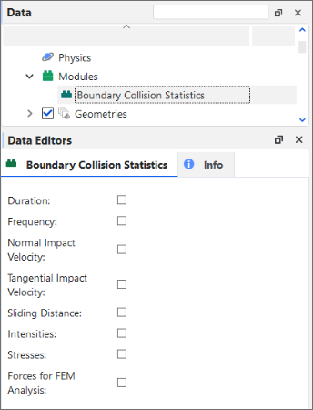
Tip: To maximize your processing capabilities, choose only the statistics that you require for your analyses.
During processing, Rocky collects the selected collision statistics between two consecutive output time levels for all boundaries in your project.
Tip: To view walk-through examples of collecting and analyzing boundary collisions statistics, refer to the following Tutorials:
Once the collisions data is collected (post-processing), specific collisions-related Properties (Figure 2) and Curves (Figure 3) will be available for the geometry or conveyor you select. (See also About Properties and About Curves.) The specific Properties and Curves available depends upon which statistics you enabled prior to processing.
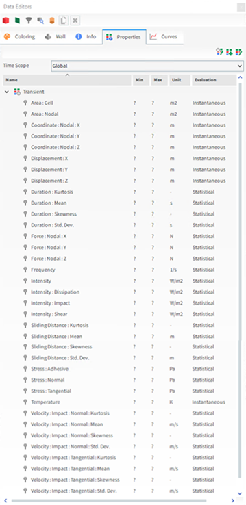
Tip: These properties will be categorized as Statistical in the Evaluation column. (See also About Viewing an Individual Statistic.)

You can then choose to analyze the resulting Properties or Curves in a plot or histogram window. (See also Graphing (Plot or Histogram) a Data Set Within Rocky)
Or, you can then choose to display the Properties information graphically on the surface of your boundaries in a 3D View window. This can be useful, for example, for showing a color map of surface intensity (Figure 3). (See also View a Color Map of Wear on the Default Belt or Imported Geometry Itself.)
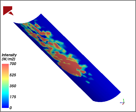
By using the Properties tab for the geometry, the options on the Coloring tab, and/or by using the slider on the Time toolbar (see also About the Time Toolbar), you can change how the data appears in the window. Tip: You may also limit your data further by using Time Statistics Properties. (See also About Adding and Editing Time Statistics Properties.)
Tip: Learn more by referring to the "Collision statistics" section in the DEM Technical Manual. (From the Rocky Help menu, point to Manuals, and then click DEM Technical Manual.)
Use Figure 1 above and the table below to understand how to collect collision statistics for your boundaries.
Table 1: Modules, Boundary Collision Statistics parameter definitions
Setting | Description | Range |
|---|---|---|
Duration | When enabled, Rocky will collect the mean, standard deviation, skewness, and kurtosis values of the duration of the collisions recorded in different regions of the geometry, during an interval between two consecutive output times. This can be useful when you are able to relate the duration to the amount of mass or heat transferred, for instance, in simulations involving chemical reactions and/or heat transfer. | Turns on or off |
Forces for FEM Analysis | When enabled, Rocky will collect the average force in various directions for each individual geometry node. This can be useful for analyzing directional forces, or side thrust. | Turns on or off |
Frequency | When enabled, Rocky will collect the average collision frequency recorded in different regions of the geometry, during an interval between two consecutive output times. This can be useful for analyzing shot flow, or for understanding the distribution of the frequency of the collisions against the surface triangles. | Turns on or off |
Intensities | When enabled, Rocky will collect the average dissipation and impact power values measured by each individual geometry triangle. This can be useful for analyzing impact wear or power draw. | Turns on or off |
Normal Impact Velocity | When enabled, Rocky will collect the mean, standard deviation, skewness, and kurtosis values of the impact relative velocity in the normal direction resulting from the collisions recorded in different regions of the geometry, during an interval between two consecutive output times. This can be useful for analyzing impact wear. | Turns on or off |
Sliding Distance | When enabled, Rocky will collect the mean, standard deviation, skewness, and kurtosis values of the sliding distance, which is the distance that a particle moves during a collision, parallel to the boundary triangle plane where the collision occurs. This can be useful for analyzing shear wear. | Turns on or off |
Stresses | When enabled, Rocky will collect the adhesion (if applicable; see note), normal and tangential stress values measured by each individual geometry triangle. This can be useful for analyzing the distribution of load due to particle collisions on a geometry. Note: Adhesive stresses are collected only when an Adhesive Force model (other than None) is enabled (see also About Physics Parameters), and an Adhesive Force Fraction for a boundary-boundary and/or boundary-particle Materials Interaction pair has a value set higher than zero (see also About Modifying Materials Interactions and Adhesion Values). | Turns on or off |
Tangential Impact Velocity | When enabled, Rocky will collect the mean, standard deviation, skewness, and kurtosis values of the impact relative velocity in the tangential direction resulting from the collisions recorded in different regions of the geometry, during an interval between two consecutive output times. This can be useful for analyzing impact wear. | Turns on or off |
What would you like to do next?
Learn more about how to Add and Edit Geometry Components
Learn more About Collecting Data in Rocky
Analyzing collision statistics for boundaries (see also About Collision Statistics for Boundaries) involves turning on the collection of the collision properties you want prior to processing your simulation.
After processing, you are then able to analyze the resulting Properties and/or Curves as you normally would.
Set up the simulation as you normally would. (See also Set Simulation Parameters.)
Before processing your simulation, do all of the following:
From the Data panel, select Modules, and then from the Data Editors panel, select Boundary Collision Statistics.
From the Data panel, under Modules, select the new Boundary Collision Statistics entry.
From the Data Editors panel, select the checkboxes for the type of statistics you want collected. (See also About Collision Statistics for Boundaries.)
Verify that the default conveyor or imported geometry has its Triangle Size set small enough to enable the detail you want. (0.1 m is recommended for most chutes and mills). (From the Data panel under Geometry, select the component you want to verify. From the Data Editors panel, on the Geometry sub-tab, verify the Triangle Size value.)
Process the simulation as you normally would. (See also Processing a Simulation.)
From the Data panel, under Geometries, select the component that you want to analyze.
From the Data Editors panel, select either the Properties or the Curves tab.
Create a plot (see also Graph Data within Rocky by Creating a Plot or Histogram) or visualize the data in a 3D View window (see also About 3D View Windows). Tips:
With Properties, you can also choose to View a Color Map of Wear on the Default Belt or Imported Geometry Itself.
You may also limit your data further by using Time Statistics Properties. (See also About Adding and Editing Time Statistics Properties.)
See Also:
In Rocky, some Particles data is collected automatically and some data you must first opt in to collecting before you process your simulation. In addition, some Particles data is always collected right from the start of the simulation, and some data waits to be collected until passing certain thresholds that you define.
Use the topics below to help you understand what, how, and when Particles data is collected in Rocky.
If you want to analyze the effects of collisions upon various particle-particle or particle-boundary pair groups within your simulation, you can choose to collect Inter-group Collision Statistics prior to processing your simulation.
Because collecting collisions statistics can take more processing time, memory, and disk storage due to increased file sizes, Rocky enables you to select from one or more sub-categories of statistics to collect. These are made available through the Inter-group Collision Statistics Module (Figure 1).
Figure 2.48: Options in the Data Editors panel when the Inter-group Collision Statistics Module is enabled
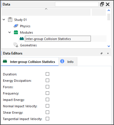
In addition, only particles and geometries belonging to particle groups and geometry components that have been enabled for Inter-group Collision Statistics collection will be recorded (Figures 2 and 3).
Figure 2.49: Additional module options for Particle groups when the Inter-group Collision Statistics module is enabled

Figure 2.50: Additional module options for a geometry component when the Inter-group Collision Statistics module is enabled
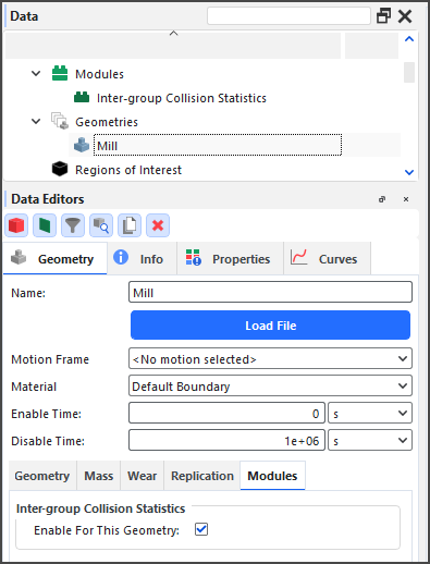
Tip: To maximize your processing capabilities, choose only the statistics that you require for your analyses.
During processing, Rocky collects the selected collision statistics between two consecutive output time levels for each participating particle-particle and particle-boundary pair.
Once the collisions data is collected (post-processing), specific collisions-related Curves (Figure 2) will be available for the main Particles entity. (See also About Curves.)
Figure 2.51: Curves for Particles (simulation-wide) when Inter-group Collision Statistics are enabled

Note: For all Inter-group Collisions Statistics curves, the effects of upscaling will be ignored for any meshed particles with Meshed Particles Upscaling enabled. (See also About Meshed Particles Upscaling.)
You can then choose to analyze the resulting Curves in a time or cross plot window. (See also Graphing (Plot or Histogram) a Data Set Within Rocky.)
Tip: Learn more by referring to the "Collision statistics" section in the DEM Technical Manual. (From the Rocky Help menu, point to Manuals, and then click DEM Technical Manual.)
Use Figure 1 above and the table below to understand how to collect Inter-group Collision Statistics.
Table 1: Modules, Inter-group Collision Statistics parameter definitions
Setting | Description | Range |
|---|---|---|
Duration | When enabled, Rocky will collect the mean, standard deviation, skewness, and kurtosis values of the duration of the collisions recorded for each particle-particle and particle-boundary pair in the simulation. | Turns on or off |
Energy Dissipation | When enabled, Rocky will collect the energy dissipation values of the collisions recorded for each particle-particle and particle-boundary pair in the simulation. | Turns on or off |
Forces | When enabled, Rocky will collect the average force in both the normal and tangential directions of the collisions recorded for each particle-particle and particle-boundary pair in the simulation. | Turns on or off |
Frequency | When enabled, Rocky will collect the average frequency of the collisions recorded for each particle-particle and particle-boundary pair in the simulation. | Turns on or off |
Impact Energy | When enabled, Rocky will collect impact energy values of the collisions recorded for each particle-particle and particle-boundary pair in the simulation. | Turns on or off |
Normal Impact Velocity | When enabled, Rocky will collect the mean, standard deviation, skewness, and kurtosis values of the impact relative velocity in the normal direction of the collisions recorded for each particle-particle and particle-boundary pair in the simulation. | Turns on or off |
Shear Energy | When enabled, Rocky will collect shear energy values of the collisions recorded for each particle-particle and particle-boundary pair in the simulation. | Turns on or off |
Tangential Impact Velocity | When enabled, Rocky will collect the mean, standard deviation, skewness, and kurtosis values of the impact relative velocity in the tangential direction of the collisions recorded for each particle-particle and particle-boundary pair in the simulation. | Turns on or off |
What would you like to do next?
See Also:
For certain solid and flexible Particle sets in Rocky (see Supported Particle Sets section below), you can choose to have collision data between two consecutive output time levels collected by Rocky during the simulation. In this version of Rocky, this is referred to as Intra-particle Collision Statistics.
Because collecting collisions statistics can take more processing time, memory, and disk storage due to increased file sizes, Rocky enables you to select from one or more sub-categories of statistics to collect. These are made available through the Intra-particle Collision Statistics Module (Figure 1).
Figure 2.52: Options in the Data Editors panel when the Intra-particle Collision Statistics Module is enabled
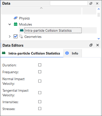
Tip: To maximize your processing capabilities, choose only the statistics that you require for your analyses.
During processing, Rocky collects the selected collision statistics between two consecutive output time levels for all applicable particle sets in your project.
Tip: To see a walk-through example of collecting and analyzing Intra-particle collisions statistics, refer to Tutorial - Tablet Coater in the Rocky Tutorial Guide.
This feature works only with Particle sets that have the following characteristics:
Single size (or monosized) only. (No particle size distributions (PSDs).)
Unbroken shapes only. (No breakage modeling.)
For Solids, Polyhedron or Custom Polyhedrons (either concave or convex) shapes only; can be either rigid or flexible, however. (No Spheres nor any type of Sphero-shapes; no Briquettes nor Faceted Cylinder shapes.)
For Fibers, flexible shapes only. (No single-element Fiber compositions. No Shell shapes of any kind, neither rigid nor flexible.)
(See also About Adding and Editing Particle Sets.)
Note: When used with Multi-Element (meshed) particles with Meshed Particles Upscaling enabled, Intra-particle Collision Statistics properties will be provided but the effects of upscaling will be ignored. This means that rather than providing data for the whole particle, data will be provided for each individual Element. (See also About Meshed Particles Upscaling.)
If you choose to enable Intra-particle Collision Statistics, then you must have at least one Particle set in your simulation that meets the above criteria. Otherwise, Rocky will not process the simulation, and you might see the following error:
Figure 2.53: Rocky error shown if no particle sets in the simulation support Intra-particle Collisions Statistics
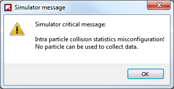
If you see this error after attempting to process your simulation, either disable Intra-particle Collision Statistics, or add a particle set that supports this type of collection.
Once the collisions data is collected (post-processing), specific collisions-related Properties (Figure 3) will be available for the supported particle set you select. (See also About Properties.) The specific Properties available depends upon which statistics you enabled prior to processing.
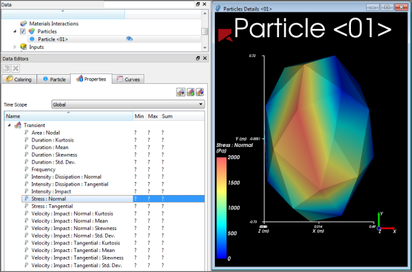
Tip: These properties will be categorized as Statistical in the Evaluation column. (See also About Viewing an Individual Statistic.)
Tip: Although it is possible to visualize the data at any time during processing, it is recommended that you avoid analyzing the data until the simulation reaches the point during which the particles are nearly constant (steady state). This is because the resulting data will have little meaning if the number of particles has a lot of variation.
You can then choose to display the collisions data graphically on the surface of a representative particle in the Particles Details window (Figure 3).
By using the slider on the Time toolbar (see also About the Time Toolbar), you can see how the data changes at different points in time.
Note: Because the Thermal Model considers a uniform temperature per individual particle, collision statistics cannot account for temperature. As a result, the Temperature property will not be available to view in a Particles Details window. However, in Collisions Statistics simulations that have both the Thermal Model enabled and use thermal-supported shape types (see also Particle and Input Limitations), you can still view the Temperature property from the main Particles entity, or from a 3D View window. (See also Enable Thermal Modeling Calculations.)
In the collision statistics visualization, a value displayed at a given vertex
is representative of all collisions in the region of influence of the vertex that
occurred in all enabled particles of the particle set being analyzed, during the time
lapse between two output time levels. This means that data displayed at time
 is the result of the statistics of the collision that happened
between time
is the result of the statistics of the collision that happened
between time  and
and  , where
  is the output period.
As usual in these type of representations, values displayed at other, non-vertex points of the particle are obtained by interpolation of available values from the surrounding vertices.
In order to get a statistical value per particle, the collision statistics that happened during that output is divided by the number of enabled particles at the time when the statistics are displayed. Therefore, it is important that these statistics should be used only when you have reached a point during the simulation where the number of particles during that output is nearly constant.
Otherwise, for example, suppose you have 100 particles from the beginning of the output period to the middle of it, and at the last time step of the output period, you have only 1 particle. The statistics of all 100 particles that were there will be divided by 1 (the number of particles at the final time step of that output period), giving values much higher than expected.
Conversely, if you get these statistics at the beginning of your simulation and particles are entering, for example, you may have 0 particles at the beginning of the first output period and 1000 particles at the end. In this case, the collision statistics will be divided by 100 and will give values much smaller than expected.
Tip: Learn more by referring to the "Collision statistics" section in the DEM Technical Manual. (From the Rocky Help menu, point to Manuals, and then click DEM Technical Manual.)
Tip: To see a walk-through example of gathering and displaying collision statistics for particles, review Tutorial - Tablet Coater in the Rocky Tutorial Guide.
Use Figure 1 above and the table below to understand how to collect Intra-particle Collisions Statistics.
Table 1: Modules, Intra-particle Collisions Statistics parameter definitions
Setting | Description | Range |
|---|---|---|
Duration | When enabled, Rocky will collect the mean, standard deviation, skewness, and kurtosis values of the duration of the collisions recorded in different regions of the representative particle of the selected particle set, during an interval between two consecutive output times. This can be useful when you are able to relate the duration to a certain process, such as in simulations involving chemical reactions and/or heat transfer. | Turns on or off |
Frequency | When enabled, Rocky will collect the average collision frequency recorded in different regions of the representative particle of the selected particle set, during an interval between two consecutive output times. This can be useful for analyzing the distribution of the frequency of the collisions around the particle surface. | Turns on or off |
Intensities | When enabled, Rocky will collect the power transferred per unit area in different regions of the representative particle of the selected particle set. Specifically:
This can be useful for evaluating the impact work around the particle, perhaps to help avoid exaggerated wear in a certain region of the particle, for example. | Turns on or off |
Normal Impact Velocity | When enabled, Rocky will collect the mean, standard deviation, skewness, and kurtosis values of the impact relative velocity in the normal direction resulting from the collisions recorded in different regions of the representative particle of the selected particle set, during an interval between two consecutive output times. This can be useful when analyzing particle breakage or granules de-agglomeration, for example. | Turns on or off |
Stresses | When enabled, Rocky will collect the adhesion (if applicable; see note), normal and tangential stress values measured by different regions of the representative particle of the selected particle set. This can be useful for analyzing damage to the particle surface due the action of concentrated forces in certain regions. Note: Adhesive stresses are collected only when an Adhesive Force model (other than None) is enabled (see also About Physics Parameters), and an Adhesive Force Fraction for a particle-boundary and/or particle-particle Materials Interaction pair has a value set higher than zero (see also About Modifying Materials Interactions and Adhesion Values). | Turns on or off |
Tangential Impact Velocity | When enabled, Rocky will collect the mean, standard deviation, skewness, and kurtosis values of the impact relative velocity in the tangential direction resulting from the collisions recorded in different regions of the representative particle of the selected particle set, during an interval between two consecutive output times. This can be useful when analyzing particle breakage or granules de-agglomeration, for example. | Turns on or off |
What would you like to do next?
If you want to expand the set of particle properties available for post-processing, including several statistical properties that may be collected during a simulation, you can choose to collect Inter-particle Collision Statistics prior to processing your simulation.
These can be useful when you need to extract data considering all collisions that happened to a certain particle between two output periods. For example, with impact velocity, you could relate that data to the chances of the particle breaking or causing it to de-agglomerate. With duration, you could relate that data to a certain mass or heat transfer process, or to a certain chemical reaction.
Because collecting collisions statistics can take more processing time, memory, and disk storage due to increased file sizes, Rocky enables you to select from one or more sub-categories of statistics to collect. These are made available through the Inter-particle Collision Statistics Module (Figure 1).
Figure 2.55: Options in the Data Editors panel when the Inter-particle Collision Statistics Module is enabled
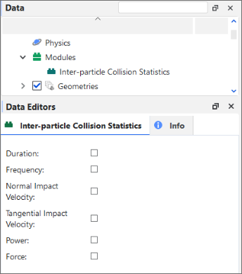
Tip: To maximize your processing capabilities, choose only the statistics that you require for your analyses.
During processing, Rocky collects the selected collision statistics between two consecutive output time levels for all particles in your project.
Note: Some Inter-particle Collision Statistics properties will not be provided for Multi-Element (meshed) particles if the Meshed Particles Upscaling feature is enabled. (See also About Meshed Particles Upscaling.)
Tip: To see a walk-through example of collecting and analyzing Inter-particle collisions statistics, refer to Tutorial - Tablet Coater in the Rocky Tutorial Guide.
Once the collisions data is collected (post-processing), specific collisions-related Properties (Figure 2) will be available for the main Particles entity. (See also About Properties.) The specific Properties available depends upon which statistics you enabled prior to processing.
Figure 2.56: Properties available for the main Particles entity when Inter-particle Collision Statistics is enabled

Tip: These properties will be categorized as Statistical in the Evaluation column. (See also About Viewing an Individual Statistic.)
You can then choose to analyze the resulting Properties in a plot or histogram window. (See also Graphing (Plot or Histogram) a Data Set Within Rocky.)
Or, you can choose to display the Properties information in a 3D View window. (See also About 3D View Windows.)
By using the Properties tab for the main Particles entity, the options on the Coloring tab, and/or by using the slider on the Time toolbar (see also About the Time Toolbar), you can change how the data appears in the window.
Tip: Learn more by referring to the "Collision statistics" section in the DEM Technical Manual. (From the Rocky Help menu, point to Manuals, and then click DEM Technical Manual.)
Use Figure 1 above and the table below to understand how to collect Inter-particle Collision Statistics.
Table 1: Modules, Inter-particle Collision Statistics parameter definitions
Setting | Description | Range |
|---|---|---|
Duration | When enabled, Rocky will collect the mean, standard deviation, skewness, and kurtosis values of the duration of the collisions recorded for each individual whole particle or fragment, during an output timestep. This can be useful when you are able to relate the duration to a certain process, such as in simulations involving chemical reactions and/or heat transfer. For example, when a homogeneous system is desired, you might seek similar collision durations across particles to help ensure a uniform distribution of the transferred quantity. Note: To make use of this property with Multi-Element (meshed) particles, the Meshed Particles Upscaling feature must be disabled. (See also About Meshed Particles Upscaling.) | Turns on or off |
Force | When enabled, Rocky will collect the sum of the forces in both the Normal and Tangential directions and for adhesion (if applicable; see note) as recorded for each individual whole particle or fragment. Note: Adhesive forces are collected only when an Adhesive Force model (other than None) is enabled (see also About Physics Parameters), and an Adhesive Force Fraction for a particle-boundary and/or particle-particle Materials Interaction pair has a value set higher than zero (see also About Modifying Materials Interactions and Adhesion Values). | Turns on or off |
Frequency | When enabled, Rocky will collect the average collision frequency recorded for each individual whole particle or fragment, during an output timestep. | Turns on or off |
Normal Impact Velocity | When enabled, Rocky will collect the mean, standard deviation, skewness, and kurtosis values of the impact relative velocity in the normal direction resulting from the collisions recorded for each individual whole particle or fragment, during an output timestep. Note: To make use of this property with Multi-Element (meshed) particles, the Meshed Particles Upscaling feature must be disabled. (See also About Meshed Particles Upscaling.) | Turns on or off |
Power | When enabled, Rocky will collect the dissipation and impact power values resulting from the collisions recorded for each individual whole particle or fragment, during an output timestep. | Turns on or off |
Tangential Impact Velocity | When enabled, Rocky will collect the mean, standard deviation, skewness, and kurtosis values of the impact relative velocity in the tangential direction resulting from the collisions recorded for each individual whole particle or fragment, during an output timestep. Note: To make use of this property with Multi-Element (meshed) particles, the Meshed Particles Upscaling feature must be disabled. (See also About Meshed Particles Upscaling.) | Turns on or off |
What would you like to do next?
For most CFD Coupling options where the fluid flow affects the motion of the particles (1-Way Constant, 1-Way Fluent, and 2-Way Fluent), you can choose to collect CFD Coupling Particle Statistics prior to processing your simulation.
These can be useful when you need to extract data considering the fluid effects upon a particle between two output periods.
Important: The 2-Way Fluent Semi-Resolved method does not compute the forces individually. Therefore, when this module is enabled within a 2-Way Fluent Semi-Resolved case, it will not return the fluid forces.
Because collecting statistics can take more processing time, memory, and disk storage due to increased file sizes, Rocky enables you to select from one or more sub-categories of statistics to collect. These are made available through the CFD Coupling Particle Statistics Module (Figure 1).
Figure 2.57: Options in the Data Editors panel when the CFD Coupling Particle Statistics Module is enabled
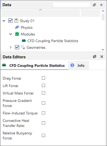
Tip: To maximize your processing capabilities, choose only the statistics that you require for your analyses.
During processing, Rocky collects the selected fluid-related statistics between two consecutive output time levels for all particles in your project.
Once the data is collected (post-processing), specific fluid-related Properties (Figure 2) will be available for the main Particles entity. (See also About Properties.) The specific Properties available depend upon which statistics you enabled prior to processing.
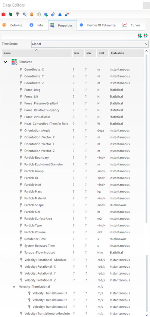 Figure 2: Properties available for the main Particles entity when CFD Coupling Particle Statistics is enabled
Tip: These properties will be categorized as Statistical in the Evaluation column. (See also About Viewing an Individual Statistic.)
You can then choose to analyze the resulting Properties in a plot or histogram window. (See also Graphing (Plot or Histogram) a Data Set Within Rocky.)
Or, you can choose to display the Properties information in a 3D View window. (See also About 3D View Windows.)
By using the Properties tab for the main Particles entity, the options on the Coloring tab, and/or by using the slider on the Time toolbar (see also About the Time Toolbar), you can change how the data appears in the window.
Use Figure 1 above and the table below to understand how to collect Fluid-Related Statistics for Particles.
Table 1: Modules, CFD Coupling Particle Statistics parameter definitions
Setting | Description | Range |
|---|---|---|
Convective Heat Transfer Rate | When enabled, Rocky will collect the average convective heat transfer rate exchanged between a particle and the surrounding fluids as recorded for each individual whole particle or fragment. Note: Data is collected only when the Thermal Model is enabled and a Convective Heat Transfer Law has been defined for the fluid-particle interactions. | Turns on or off |
Drag Force | When enabled, Rocky will collect the average drag force applied by fluids as recorded for each individual whole particle or fragment. | Turns on or off |
Flow-Induced Torque | When enabled, Rocky will collect the average torque induced by fluid flow as recorded for each individual whole particle or fragment. Note: Data is collected only when a Torque Law has been defined for the fluid-particle interactions. | Turns on or off |
Lift Force | When enabled, Rocky will collect the average lift force applied by fluids as recorded for each individual whole particle or fragment. Note: Data is collected only when a Lift Law has been defined for the fluid-particle interactions. | Turns on or off |
Pressure Gradient Force | When enabled, Rocky will collect the average pressure gradient force applied by fluids as recorded for each individual whole particle or fragment. | Turns on or off |
Virtual Mass Force | When enabled, Rocky will collect the average virtual mass force applied by fluids as recorded for each individual whole particle or fragment. Note: Data is collected only when a Virual Mass Law has been defined for the fluid-particle interactions. | Turns on or off |
What would you like to do next?
If you want to perform global or partial energy balances in a simulation, you can choose to collect particle instantaneous energies prior to processing your simulation, which enables the calculation of the kinetic and potential energies of each individual particle in the simulation.
You choose to collect these kind of particle energies by enabling the Particle Instantaneous Energies Module (Figure 1).
Figure 2.58: There are no options in the Data Editors panel when the Particle Instantaneous Energies Module is enabled
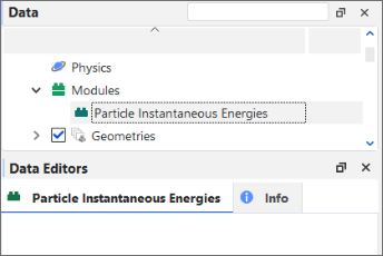
During processing, Rocky collects particle energies data for each particle based upon its translational/rotational velocity and position in space.
Once the energies data is collected (post-processing), specific energy-related Properties (Figure 2) and Curves (Figure 3) will be available for the main Particles entity. (See also About Properties and About Curves.)
Figure 2.59: Properties for Particles (simulation-wide) when Particle Instantaneous Energies is enabled
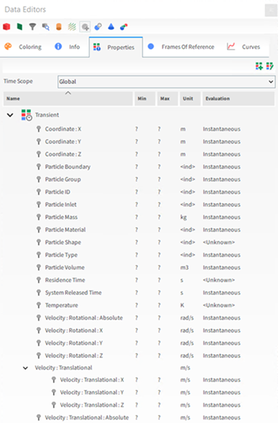
These Properties are based on the following energies calculations:
Translational kinetic energy: The energy related to the rectilinear motion of a particle. It is given by:
 where:
  is the particle's mass, and
  is the velocity of its center of mass.
 Rotational kinetic energy: This is the energy due to the rotation of a particle around an axis through its center of mass. It is given by:
 where:
  is the particle's angular velocity, and
  is the moment of inertia tensor.
 Potential energy: This is the energy of a particle due to its position relative to the Earth's gravitational field. In Rocky it is calculated as:
 where:
  is the particle's mass,
  is the acceleration due to gravity, and
  is the position vector of the particle's center of mass.
Conventionally, a zero potential energy is attributed to a plane orthogonal to the
gravity direction, passing through the origin of the coordinate system.
is the position vector of the particle's center of mass.
Conventionally, a zero potential energy is attributed to a plane orthogonal to the
gravity direction, passing through the origin of the coordinate system.
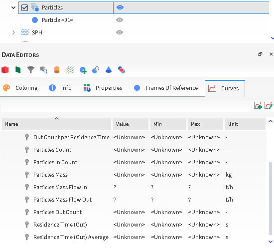
The Energy Delta Curve represents a variation (delta) in total energy of the particles recorded during an interval between two consecutive output times.
You can choose to visualize the resulting Properties and Curves in a 3D View window (Figure 3), or analyze the results in a time or other plot window. (See also Graphing (Plot or Histogram) a Data Set Within Rocky.)

What would you like to do next?
See Also:
Analyzing Inter-group Collision Statistics for each particle-particle or particle-boundary pair group (see also About Inter-group Collision Statistics) involves turning on the collection of the collision properties you want prior to processing your simulation, and then determining which particle groups and geometries you want to involve in that collection.
After processing, you are then able to analyze the resulting Curves.
Set up the simulation as you normally would. (See also Set Simulation Parameters.)
Before processing your simulation, do all of the following:
From the Data panel, select Modules, and then from the Data Editors panel, select the Inter-group Collision Statistics checkbox.
From the Data panel, under Modules, select the new Inter-group Collision Statistics entry.
From the Data Editors panel, select the checkbox for each type of statistics you want collected. (See also About Inter-group Collision Statistics.)
For each geometry component that you do not want included in the collection of Inter-group Collision Statistics, do the following:
From the Data panel, under Geometries select the geometry that you want to exclude from Inter-group Collision Statistics collections.
From the Data Editors panel, select the Geometry | Modules tab and then under Inter-group Collision Statistics clear the Enable For This Geometry checkbox.
For each particle group that you do not want included in the collection of Inter-group Collision Statistics, do the following:
From the Data panel, under Particles select the particle group that you want to exclude from Inter-group Collision Statistics collections.
From the Data Editors panel, select the Particle | Modules tab and then under Inter-group Collision Statistics clear the Enable For This Particle Group checkbox.
Process the simulation as you normally would. (See also Processing a Simulation.)
From the Data panel, select the main Particles entity.
From the Data Editors panel, select the Curves tab.
Create a time or cross plot. (See also Graph Data within Rocky by Creating a Plot or Histogram.)
See Also:
Analyzing collision statistics for particle surfaces involves first turning on the collection of Intra-particle Collision Statistics prior to processing the simulation (see also About Intra-Particle Collision Statistics), and then viewing the resulting Properties for a supported Particle set on the surface of a representative particle in a Particles Details window.
By using the slider on the Time toolbar (see also About the Time Toolbar), you can see how the data changes at different points in time.
Set up your simulation as you normally would (see also Setting Up a Simulation). Note: If you decide to enable the Thermal Model, know that while the Temperature property will not be available to view on the Particles Details window, it can still be viewed from the main Particles entity or through a 3D View window. (See also Enable Thermal Modeling Calculations.)
Before processing your simulation, do all of the following:
From the Data panel, select Modules, and then from the Data Editors panel, select the Intra-particle Collision Statistics checkbox.
From the Data panel, under Modules, select the new Intra-particle Collision Statistics entity.
From the Data Editors panel, enable the checkboxes for the type of statistics you want collected. (See also About Intra-Particle Collision Statistics.)
Ensure you have added at least one Particle set that is eligible for intra-particle collision statistics collection. Note: Intra-particle collision statistics can be collected only on single sized particle sets that have no breakage enabled and that make use of the following shapes:
Polyhedron (rigid or flexible)
Custom Polyhedron (convex or concave, rigid or flexible)
Straight Fiber or Custom Fiber (flexible only)
(See also About Adding and Editing Particle Sets.)
Process your simulation as you normally would (see also About Starting a Simulation.)
From the Data panel, under Particles, select the Particle set for which you want to view intra-particle collision statistics, and then click the View button. A new Particles Details window opens showing a particle that represents the whole Particle set.
Display intra-particle collision statistics Properties on the view in one of the following ways:
From the Properties tab, click a Property and then drag and drop it on the Particles Details window. (See also About Properties.) Tips: You may also make use of Time Statistics Properties. (See also About Adding and Editing Time Statistics Properties.)
From the Coloring tab, use the Property lists to change what is colored in the Particles Details window. (See also Use the Coloring Tab to Change the Preview for a Particle Set.)
Use the slider on the Time toolbar to change what timestep is displaying data. (See also About the Time Toolbar.) Note: The data displayed at a given timestep was collected in the interval between that timestep and the previous one.
Tips:
Use your mouse to zoom, pan, and rotate the view, just as you would in a 3D View window. (See also Use the Mouse, Keyboard, or Toolbar to Change a 3D View.)
Change the look of the window by right-clicking the window, or by using the options on the Windows Editors panel. (See also About Using the Window Editors Panel to Change the Selected Particles Details Window.)
See Also:
Analyzing inter-particle collision statistics (see also About Inter-particle Collision Statistics) involves turning on the collection of the collision properties you want prior to processing your simulation.
After processing, you are then able to analyze the resulting Properties as you normally would.
Set up the simulation as you normally would. (See also Set Simulation Parameters.)
Before processing your simulation, do all of the following:
From the Data panel, select Modules, and then from the Data Editors panel, enable the Inter-particle Collision Statistics checkbox.
From the Data panel, under Modules, select the new Inter-particle Collision Statistics entry, and then from the Data Editors panel, enable the checkboxes for the type of statistics you want collected. (See also About Inter-particle Collision Statistics.)
Process the simulation as you normally would. (See also Processing a Simulation.)
From the Data panel, select the main Particles entity.
From the Data Editors panel, select the Properties tab.
Create a plot (see also Graph Data within Rocky by Creating a Plot or Histogram), or visualize the data in a 3D View window (see also About 3D View Windows).
See Also:
Analyzing Particle Instantaneous Energies (see also About Particle Instantaneous Energies) involves turning on the collection of energies data prior to processing your simulation.
After processing, you are then able to analyze the resulting Properties as you normally would.
Set up the simulation as you normally would. (See also Set Simulation Parameters.)
Before processing your simulation, do all of the following:
From the Data panel, select Modules.
From the Data Editors panel, select the Particle Instantaneous Energies checkbox.
Process the simulation as you normally would. (See also Processing a Simulation.)
From the Data panel, select the main Particles entity.
From the Data Editors panel, select the Properties tab.
Create a 3D View (see also View Geometries, Particles, Points, and Fluids in 3D) or plot (see also Graph Data within Rocky by Creating a Plot or Histogram).
See Also:
Analyzing fluid-related statistics for particles (see also About Fluid-Related Statistics for Particles) involves turning on the collection of the fluid-related properties you want prior to processing your CFD Coupling simulation.
After processing, you are then able to analyze the resulting Properties for the main Particles entity as you normally would.
Set up your CFD Coupling simulation as you normally would. (See also Set Simulation Parameters.)
Before processing your simulation, do all of the following:
From the Data panel, select Modules, and then from the Data Editors panel, enable the CFD Coupling Particle Statistics checkbox.
From the Data panel, under Modules, select the new CFD Coupling Particle Statistics entry, and then from the Data Editors panel, enable the checkboxes for the type of statistics you want collected. (See also About Fluid-Related Statistics for Particles.)
Process the simulation as you normally would. (See also Processing a Simulation.)
From the Data panel, select the main Particles entity.
From the Data Editors panel, select the Properties tab.
Create a plot (see also Graph Data within Rocky by Creating a Plot or Histogram), or visualize the data in a 3D View window (see also About 3D View Windows).
See Also:
In Rocky, contacts and energy spectra data is collected only if you first opt in to collecting them before you process your simulation. After choosing to collect it, contacts data is always collected right from the start of the simulation. However, data for energy spectra waits to be collected until passing certain thresholds that you define.
Depending on the source of the energy values considered, two types of energy spectra plots are available in Rocky: Contacts Energy Spectra and Particles Energy Spectra.
With Contacts Energy Spectra, the energy values are collected collision-wise during the simulation and the resulting data is categorized by the contact pair (particle group and/or geometry).
With Particles Energy Spectra the energy values collected during the simulation are related only to particles, and the resulting data is classified by size and particle group.
Based upon your energy analysis needs, you can use either or both types of energy spectra in your simulation.
Important: The energy scale in all energy spectra plots is logarithmic, so zero is not a valid value for the minimum energy, therefore for Contacts and Particles energy spectra the minimum energy values must be greater than zero.
Use the topics below to help you understand what, how, and when contacts and energy spectra data is collected in Rocky.
In Rocky, it is possible simulate the breakage behavior of particles. (See also Enable Particle Breakage Calculations.) However, simulations with breakage enabled can increase the computational cost, taking longer to process the simulation. With this in mind, Rocky has another feature you can use to analyze breakage: Contacts Energy Spectra.
This useful tool collects different kinds of energy statistics per contact pair (particle group and/or geometry) and size, which helps provide insight into the distribution of the energies of all collisions that occurred in a simulation up to a given time. In this version of Rocky, these statistics are collected through the Contacts Energy Spectra module (Figure 1).
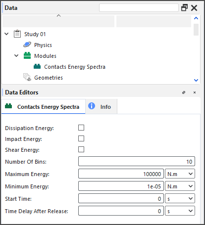
This kind of energy spectra is often used in conjunction with Particles Energy Spectra. (See also About Particles Energy Spectra.)
See the sections below for more information about this type of energy statistic, and how it is collected, calculated, and viewed in Rocky.
For contact-based analysis, the energy statistics of particle collisions are collected per collision; i.e., every separate particle-to-particle or particle-to-geometry impact will have its resulting energy collision stored. Each statistics pair-which is composed of either two Particle sets or one Particle set and one Geometry-will present a separate Energy Spectra curve. In this version of Rocky, only particles and geometries belonging to particle groups and geometry components that have been enabled for energy spectra collection will be recorded (Figures 2 and 3).
Figure 2.63: Additional module options for Particle groups when the Contacts Energy Spectra module is enabled
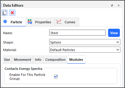
Figure 2.64: Additional module options for a geometry component when the Contacts Energy Spectra module is enabled

These curves are based upon three different types of collision energy, each of which can be useful for different types of analyses: Dissipation Energy, Impact Energy, and Shear Energy.
Because collecting statistics can take more processing time, memory, and disk storage due to increased file sizes, Rocky enables you to select which of these three collision energies you want to collect, and enables you to choose which particle groups and geometry components will participate in energy spectra collection.
It is important to realize that data is only collected after both the Start Time and Time Delay After Release values are reached. Data begins being collected at the Start Time but only for the particles that were released before the Time Delay After Release value. This is to allow enough time for the particle flow within your simulation to reach a steady state before the energy spectra calculations begin.
For example, if the Start Time is 5s, and the Time Delay After Release is 3s, a particle entering the simulation at 4s will only be accounted for after 7s of simulation time.
One common application of this type of analysis is for comminution devices like SAG mills (Figure 4), which use steel balls or other kinds of grinding media to help break rock or ore material into smaller fragments.

Although mills have great energy consumption, only a small part of this energy is converted into actual particle fragmentation. This inefficiency is mainly due to the fact that not all impacts lead to breakage. Impacts of low energy will not cause breakage, while excessive intensity impacts apply only part of the total energy to the breakage process. The rest of this energy is lost.
Therefore, it is important to understand how power is consumed during comminution processes in order to improve grinding efficiency. The Contact-based analysis is especially useful when combined with the Cumulative Power analysis for a comminution process because you can get an estimate of how collision energy is distributed amongst contacts.
In this way, by comparing contacts energy spectra per material pair for different equipment designs, higher collision energies involving the material to be broken (rock-rock, rock-ball, or rock-wall, for example) might lead to higher particle breakage. On the other hand, collision energies involving only the equipment or grinding materials (ball-ball or ball-wall, for example) could be considered wasted by not leading to particle breakage, and should be minimized through improved designs.
Contacts Energy Spectra curves can be displayed by Power, Cumulative Power (Figure 5), and Rate.
Figure 2.66: Examples of Contacts Impact Energy Spectra curves for various particle-to-particle and particle-to-geometry contact pairs
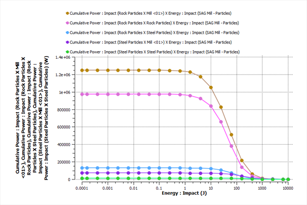
Tip: Refer to the DEM Technical Manual for implementation details. (From the Help menu, point to Manuals, and then click DEM Technical Manual.)
If prior to processing your simulation, you enabled Contacts Energy Spectra to be collected, then while the simulation is processing, Rocky calculates the selected energy curves (Dissipation, Impact, and/or Shear) for each pair of particle-to-particle or particle-to-geometry contact types, each generated by the power, cumulative power, and collisions rate (Figure 6).

You can then create a Cross plot of the Curves you are interested in analyzing (Figure 7).
Figure 2.68: Example cross plot of Contacts Energy Spectra showing both Cumulative Power and Power, for impact collisions between particles and geometries

When opening projects that were created and processed in versions of Rocky prior to 2022 R1, Rocky will still read the energy spectra data in those projects and will display the energy spectra Curves as usual.
However, if you want to modify and then re-process an older energy spectra simulation in 2022 R1 or later versions, you will need to enable the energy spectra modules and define the type of collection parameters you want prior to processing the simulation.
The same is true for projects that you have created but not processed in older versions of Rocky; you must enable and define the energy spectra modules manually before processing your simulation.
Use Figures 1-3 above and the tables below to understand how to collect contact-based energy statistics.
Table 1: Modules, Contacts Energy Spectra parameter definitions
Setting | Description | Range |
|---|---|---|
Dissipation Energy | When enabled, collects contact-based statistics for dissipation energy, which is the fraction of the mechanical energy transformed irreversibly into other forms of energy during a collision. | Turns on or off |
Impact Energy | When enabled, collects contact-based statistics for impact energy, which is the maximum energy transferred during a collision. Tip: When Rocky simulates an actual breakage process (see also Enable and View Particle Breakage), this is usually the energy type considered to quantify the damage on the particles. | Turns on or off |
Shear Energy | When enabled, collects contact-based statistics for shear energy, which is the work done by the tangential contact forces during a collision. | Turns on or off |
Number of Bins | This defines how many sub-intervals the specified energy interval is evenly (using a logarithmic scale) subdivided. Determines the the resolution of the resulting Curves. The higher the value, the better the resolution. | Positive values |
Maximum Energy | This defines the right bound of the interval of energies that will be subdivided into bins for the construction of the energy spectra Curves. | Positive values |
Minimum Energy | This defines the left bound of the interval of energies that will be subdivided into bins for the construction of the energy spectra Curves. | Positive values |
Start Time | The amount of time you want to wait before starting to register energy spectra data. Tip: It is best practice to set your Start Time to begin after a steady state has been reached in your particle flow. | Value must be positive but less than Simulation Duration, which is located on the Solver | Time sub-tab. (See also About Solver Parameters.) |
Time Delay after Release | The amount of time you want to wait after a particle has been released before starting to register energy spectra data. | Value must be positive but less than Simulation Duration, which is located on the Solver | Time sub-tab. (See also About Solver Parameters.) |
Table 2: Individual Geometry, Modules sub-tab parameter definitions
Setting | Description | Range |
|---|---|---|
Enable For This Geometry | When enabled, the energy values involving this geometry will be recorded for energy spectra purposes. When cleared, the energy values involving this geometry will be ignored. | Turns on or off |
Table 3: Individual Particle Group, Modules sub-tab parameter definitions
Setting | Description | Range |
|---|---|---|
Enable For This Particle Group | When enabled, the energy values involving particles from this group will be recorded for energy spectra purposes. When cleared, the energy values involving particles from this group will be ignored. | Turns on or off |
What would you like to do?
Learn more About Collecting Data
Learn more About Curves
See Also
In Rocky, it is possible simulate the breakage behavior of particles. (See also Enable Particle Breakage Calculations.) However, simulations with breakage enabled can increase the computational cost, taking longer to process the simulation. With this in mind, Rocky has another feature you can use to analyze breakage: Particles Energy Spectra.
This useful tool collects different kinds of energy statistics per particle type and size category defined in its PSD, which can help predict breakage and attrition rates for continuous processes such as grinding mills. In this version of Rocky, these statistics are collected through the Particles Energy Spectra module (Figure 1).
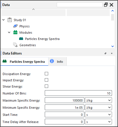
This kind of energy spectra is often used in conjunction with Contacts Energy Spectra. (See also About Contacts Energy Spectra.)
See the sections below for more information about this type of energy statistic, and how it is collected, calculated, and viewed in Rocky.
For particle-based analysis, relevant energy values associated to the collisions experienced by each individual particle collected during the simulation. In this version of Rocky, only particles belonging to particle groups that have been enabled for energy spectra collection will be recorded (Figure 2).
Figure 2.70: Additional module options for Particle groups when the Particles Energy Spectra module is enabled
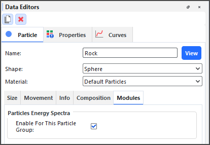
Rocky then classifies and accumulates the associated specific energy values (energy per particle mass) according to a predefined set of energy levels, and represents the resulting cumulative values as curves.
For Particles Energy Spectra analysis, each particle group and particle size category will present a separate Energy Spectra curve. These curves are based upon three different types of collision energy, each of which can be useful for different types of analyses:
Dissipation Energy, which is the particle's mechanical energy transformed irreversibly into other forms of energy during a collision.
Impact Energy, which is the energy considered in breakage models for quantifying the damage on the particle's material that can lead to breakage. Tips: When Rocky simulates an actual breakage process (see also Enable and View Particle Breakage), this is usually the energy type considered to quantify the damage on the particles.
Shear Energy, which is the energy used to predict the abrasive wear of boundaries.
Because collecting statistics can take more processing time, memory, and disk storage due to increased file sizes, Rocky enables you to select which of these three particles energies you want to collect, and enables you to choose which particle groups will participate in energy spectra collection.
It is important to realize that data is only collected after both the Start Time and Time Delay After Release values are reached. Data begins being collected at the Start Time but only for the particles that were released before the Time Delay After Release value. This is to allow enough time for the particle flow within your simulation to reach a steady state before the energy spectra calculations begin.
For example, if the Start Time is 5s, and the Time Delay After Release is 3s, a particle entering the simulation at 4s will only be accounted for after 7s of simulation time.
One common application of this type of analysis is for comminution devices like SAG mills (Figure 3), which use steel balls or other kinds of grinding media to help break rock or ore material into smaller fragments.
By looking at energy levels applied to particles, for instance, you can predict breakage rates.
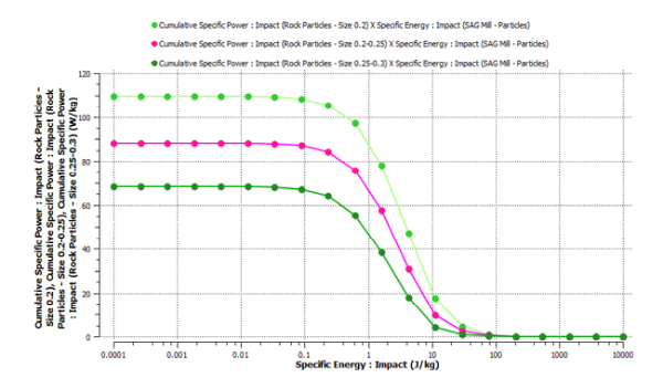
In the example shown in Figure 4 above, the Y-axis gives the Cumulative Specific Power : Impact values resulting from all collisions starting from the Start Time time you enter until the end of the simulated time (see also About Solver Parameters). The value of the Y-coordinate of a given point on the curve is obtained by dividing the cumulative specific energy by the time elapsed since the referred starting time. This value accounts for all collisions with a specific impact energy equal or higher than the specific energy given by its X-coordinate.
This kind of energy spectra curve is useful for the reason that all collisions with specific impact energy higher than a known threshold value may lead to particle breakage, while the remaining collisions will not, as shown in Figure 5 below. Therefore, the cumulative specific power available for breakage in that case will be given by the Y-coordinate in the curve, corresponding to the breakage threshold value.

Important: This threshold value is the minimum value of impact energy that can break a particle, which is a known value derived from experiments. It will therefore change depending upon the material being simulated.
Tips:
Refer to the DEM Technical Manual for implementation details. (From the Help menu, point to Manuals, and then click DEM Technical Manual.)
To see a walk-through example of particles energy spectra being using to analyze breakage in a SAG mill, review Tutorial - SAG Mill in the Rocky Tutorial Guide.
If prior to processing your simulation, you enabled Particles Energy Spectra to be collected, then while the simulation is processing, Rocky calculates the selected Cumulative Specific Power curves (Dissipation, Impact, and/or Shear) for each particle set, generated by each size of the particle size distribution, and separated by Specific Energy. These curves are grouped under Specific Energy on the Curves tab (Figure 6).
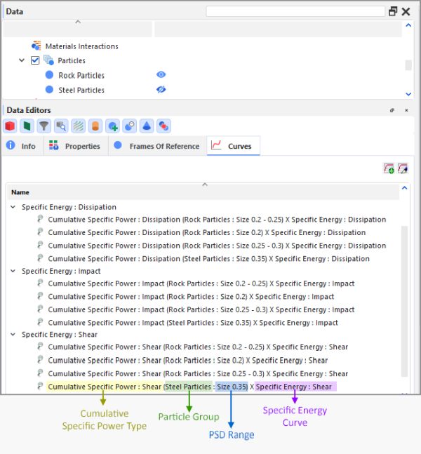
Using these curves, you can then create a Cross plot, similar to the example below (Figure 7).

When opening projects that were created and processed in versions of Rocky prior to 2022 R2, Rocky will still read the energy spectra data in those projects and will display the energy spectra Curves as usual.
However, if you want to modify and then re-process an older energy spectra simulation in 2022 R2 or later versions, you will need to enable the energy spectra modules and define the type of collection parameters you want prior to processing the simulation.
The same is true for projects that you have created but not processed in older versions of Rocky; you must enable and define the energy spectra modules manually before processing your simulation.
Use Figures 1-2 above and the tables below to understand how to collect particle-based energy statistics.
Table 1: Modules, Particles Energy Spectra parameter definitions
Setting | Description | Range |
|---|---|---|
Dissipation Energy | When enabled, collects particle-based statistics for dissipation energy, which is the fraction of the mechanical energy transformed irreversibly into other forms of energy during a collision. | Turns on or off |
Impact Energy | When enabled, collects particle-based statistics for impact energy, which is the maximum energy transferred during a collision. Tip: When Rocky simulates an actual breakage process (see also Enable and View Particle Breakage), this is usually the energy type considered to quantify the damage on the particles. | Turns on or off |
Shear Energy | When enabled, collects particle-based statistics for shear energy, which is the work done by the tangential contact forces during a collision. | Turns on or off |
Number of Bins | This defines how many sub-intervals the specified energy interval is evenly (using a logarithmic scale) subdivided. Determines the the resolution of the resulting Curves. The higher the value, the better the resolution. | Positive values |
Maximum Specific Energy | This defines the right bound of the interval of specific energies that will be subdivided into bins for the construction of the energy spectra Curves. | Positive values |
Minimum Specific Energy | This defines the left bound of the interval of specific energies that will be subdivided into bins for the construction of the energy spectra Curves. | Positive values |
Start Time | The amount of time you want to wait before starting to register energy spectra data. Tip: It is best practice to set your Start Time to begin after a steady state has been reached in your particle flow. | Value must be positive but less than Simulation Duration, which is located on the Solver | Time sub-tab. (See also About Solver Parameters.) |
Time Delay after Release | The amount of time you want to wait after a particle has been released before starting to register energy spectra data. | Value must be positive but less than Simulation Duration, which is located on the Solver | Time sub-tab. (See also About Solver Parameters.) |
Table 2: Individual Particle Group, Modules sub-tab parameter definitions
Setting | Description | Range |
|---|---|---|
Enable For This Particle Group | When enabled, the energy values involving particles from this group will be recorded for energy spectra purposes. When cleared, the energy values involving particles from this group will be ignored. | Turns on or off |
What would you like to do?
Learn more About Collecting Data
Learn more About Curves
See Also
Analyzing data for Contacts Energy Spectra involves first turning on the type of collection you want prior to processing the simulation (see also About Contacts Energy Spectra), and then determining which particle groups and geometries you want to involve in that collection. After processing your simulation you can then plot the resulting Curves (Figure 1).
It is important to realize that data is only collected after the Start Time value is reached.
For more details, tips, and limitations, see the About Contacts Energy Spectra topic.
Set up your simulation as you normally would (see also Set Simulation Parameters).
Before processing your simulation, do all of the following:
From the Data panel, select Modules, and then from the Data Editors panel, select Contacts Energy Spectra.
From the Data panel, under Modules, select the new Contacts Energy Spectra entry.
From the Data Editors panel, on the Contacts Energy Spectra tab, do all of the following:
Select one or more of the checkboxes for the type of energy statistics you want collected. (See also About Contacts Energy Spectra.) Important: You must select at least one checkbox in order for energy spectra to be collected.
In the Number of Bins box, enter the number of sub-intervals you want the energy interval to be evenly (using a logarithmic scale) subdivided.
In the Maximum Energy and Minimum Energy boxes, enter values for the right an left bounds of the interval of energies that will be subdivided into bins for the construction of the energy spectra Curves.
Set the values you want for both Start Time and Time Delay after Release. IMPORTANT: Because energy spectra is calculated as an average over time, it is important that you set this data to be collected after steady state has been reached.
For each geometry component that you do not want included in the collection of energy spectra, do the following:
From the Data panel, under Geometries select the geometry that you want to exclude from energy spectra collections.
From the Data Editors panel, select the Geometry | Modules tab and then under Contacts Energy Spectra clear the Enable For This Geometry checkbox.
For each particle group that you do not want included in the collection of energy spectra, do the following:
From the Data panel, under Particles select the particle group that you want to exclude from energy spectra collections.
From the Data Editors panel, select the Particle | Modules tab and then under Contacts Energy Spectra clear the Enable For This Particle Group checkbox.
Process your simulation as you normally would. (See also About Starting a Simulation.)
After your simulation reaches as least as far as the Start Time value, do the following:
From the Data panel, select Particles.
From the Data Editors panel, select the Curves tab.
Under the three Energy categories (Dissipation, Impact, and Shear), drag one or more of the Curves listed to the Workspace. (See also About Curves.) A new Cross Plot window is created showing the Curve(s) you selected.
From the Cross Plot window, do one or both of the following:
Modify the appearance of the Cross Plot. (See also About Changing the Appearance of a Graph (Plot or Histogram).) Tips: To show a Curve in a logarithmic format, right-click the desired axis and select Customize Axis. From the Axis tab, under Scale Options, enable the Logarithmic Scale checkbox.
Export the data to a CSV file. (See also Export Data into a CSV File.)
See Also:
Analyzing data for Particles Energy Spectra involves first turning on the type of collection you want prior to processing (see also About Particles Energy Spectra), and then determining which particle groups you want to involve in that collection. After processing your simulation you can then plot the resulting Curves (Figure 1).
It is important to realize that data is only collected after the Start Time value is reached.
For more details, tips, and limitations, see the About Particles Energy Spectra topic.
Set up your simulation as you normally would (see also Set Simulation Parameters).
Before processing your simulation, do all of the following:
From the Data panel, select Modules, and then from the Data Editors panel, select Particles Energy Spectra.
From the Data panel, under Modules, select the new Particles Energy Spectra entry.
From the Data Editors panel, on the Particles Energy Spectra tab, do all of the following:
Select one or more of the checkboxes for the type of energy statistics you want collected. (See also About Particles Energy Spectra.) Important: You must select at least one checkbox in order for energy spectra to be collected.
In the Number of Bins box, enter the number of sub-intervals you want the specific energy interval to be evenly (using a logarithmic scale) subdivided.
In the Maximum Energy and Minimum Energy boxes, enter values for the right an left bounds of the interval of specific energies that will be subdivided into bins for the construction of the energy spectra Curves.
Set the values you want for both Start Time and Time Delay after Release. IMPORTANT: Because energy spectra is calculated as an average over time, it is important that you set this data to be collected after steady state has been reached.
For each particle group that you do not want included in the collection of energy spectra, do the following:
From the Data panel, under Particles select the particle group that you want to exclude from energy spectra collections.
From the Data Editors panel, select the Particle | Modules tab and then under Particles Energy Spectra clear the Enable For This Particle Group checkbox.
Process your simulation as you normally would. (See also About Starting a Simulation.)
After your simulation reaches as least as far as the Start Time value, do the following:
From the Data panel, select Particles.
From the Data Editors panel, select the Curves tab.
Under the three Specific Energy categories (Dissipation, Impact, and Shear), drag one or more of the Curves listed to the Workspace. (See also About Curves.) A new Cross Plot window is created showing the Curve(s) you selected.
From the Cross Plot window, do one or both of the following:
Modify the appearance of the Cross Plot. (See also About Changing the Appearance of a Graph (Plot or Histogram).) Tip: To show a Curve in a logarithmic format, right-click the desired axis and select Customize Axis. From the Axis tab, under Scale Options, enable the Logarithmic Scale checkbox.
Export the data to a CSV file. (See also Export Data into a CSV File.)
See Also:
Rocky comes integrated with several Ansys products including Mechanical, Fluent, Motion, Minerva, and optiSLang.
Rocky can also integrate with Ansys Workbench. Working through Workbench enables Rocky to couple its abilities with other Ansys products - including Mechanical, Fluent, DesignXplorer, and SpaceClaim - which enables you to define design points for parametric cases, and solve more kinds of solutions in more complex and innovative ways.
When a Rocky project is connected to Ansys Mechanical though Workbench, an External Coupling component becomes enabled in the Rocky Data panel. This component enables you to define the kind of data gets shared between the programs, such as the geometry loads.
What would you like to do?
Learn more About Rocky and Ansys Workbench Integration
Learn more About Rocky and Ansys Mechanical Integration
Learn more About Rocky and Ansys Fluent Integration
Learn more About Rocky and Ansys Motion Integration
Learn more About Rocky and Ansys optiSLang Integration
Learn more About Rocky and Ansys Minerva Integration
See Also:
Ansys Workbench is a product you can use to more easily connect, share, automate, and keep organized data across various programs. When used with Rocky, Workbench can help you accomplish many time-saving tasks like the ones described in the sections below.
Tip: To learn which versions of Ansys-including Workbench, SpaceClaim, Mechanical, Fluid, and other products-are compatible with this version of Rocky, refer to System Requirements.
This is accomplished through Workbench by connecting your Rocky project with Ansys SpaceClaim 3D geometry files, thereby enabling you to change equipment components in SpaceClaim (Figure 1) and have those geometry changes be automatically updated in your Rocky project.
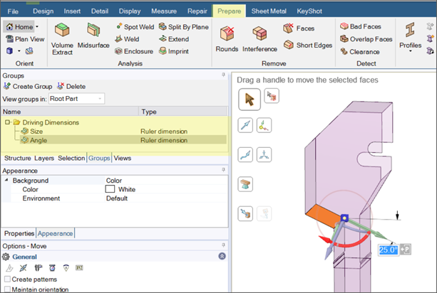
Tip: To see walk-through examples of modifying your geometries in SpaceClaim for use in your Workbench-connected Rocky projects, refer to the following Tutorials:
This is accomplished through Workbench by connecting your Rocky project with Ansys DesignXplorer, which enables you to set design goals and get immediate feedback on proposed changes. DesignXplorer includes correlation, design of experiments, response surface creation and analysis, optimization and six sigma analysis. In addition, integration with other Ansys products like SpaceClaim ensures that any geometry changes made are automatically updated in your Rocky project.
An example of such a project is shown in Figure 2 where varied geometrical inputs as well as Rocky inputs are used to evaluate the impact of those changes in Rocky output parameters. (See also About Defining and Using Input Variables and About Defining Output Variables.)
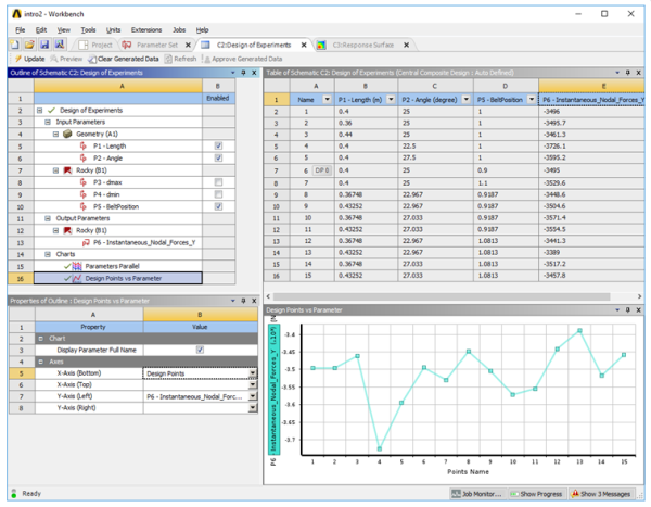
Using DesignXplorer through Workbench can be especially helpful when testing how small changes in geometry angles, sizes, or placements affects your material flow.
By using Workbench to connect your Rocky project with Ansys Mechanical, you can have Mechanical predict the stress and strain response of your geometry components when they are subjected to the granular loads that are calculated in Rocky.
Workbench does this by first having Rocky calculate the particle forces and pressures on the geometry component. Next, it automatically exports that data from Rocky to Mechanical through Workbench, where Mechanical then uses those forces and pressures to perform static (at a single time - Figure 3) or transient (over a time range - Figure 4) structural analysis on the component.
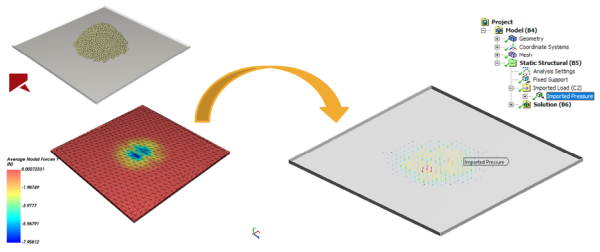
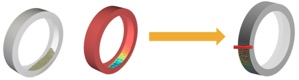
This approach is useful for analyzing the stress effects of particles upon a vibrating screen, for example, or for visualizing the mechanical deformation of a bucket excavator due to particle loads.
Tip: To learn more about using Mechanical to conduct Static and Transient FEA analyses in your Workbench-connected Rocky projects, refer to the following resources:
By using Workbench to couple your Rocky project 1-Way with Ansys Fluent, Rocky can calculate how the CFD fluid flow and heat transfer affects the DEM particle flow and related thermal properties (Figure 5).
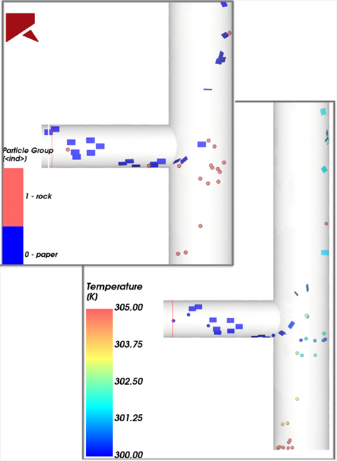
This approach is useful for studying how air flow affects various kinds of material flowing through a pipe, for example.
Tip: To see a walk-through example of a 1-Way coupled simulation with Ansys Fluent, refer to the following Tutorial: Tutorial 13 - DEM-CFD One Way Coupling With Ansys Fluent (Workbench).
From Rocky 23R1 it's possible to use both 1-way and 2-way CFD-DEM coupling analyses through Ansys Workbench. This functionality brings many advantages, such as:
Multiphysics Analyses Integration: With a single interface, it's possible to integrate multiple analyses, making it easy to see in the workflow project who is sending data to whom.
Automated Data Management: Save time without the need to manually transfer the results from one application to another.
Run multiple designs: to explore different scenarios.
Optimizing Exploration: parametric modeling capabilities in conjunction with optimization techniques to allow you to efficiently investigate the effects of input parameters on selected output parameters.
Workflow: all the necessary files are archived together, making it easy to share the project with other users.
To couple Rocky and Fluent in Workbench, follow the steps below:
The 1-way coupling can use either a steady or transient flow field. For the 1-way coupling, select Fluent Solution Properties and change the Initialization Method to Solver Controlled;
Figure 2.83: For 1-way coupled simulations, the Initialization Method should be set as "Solver Controlled" in the Fluid Flow Solution Properties.
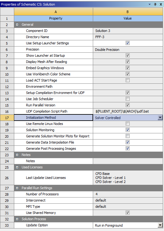
For a 1-way transient coupling, the option to Export the transient data must be enabled in the Rocky Export entry in Fluent.
To use the flow field in the 1-way coupled simulation, link the Fluent Solution to the Rocky Setup.
For sharing the geometry between projects, link the Geometry of the Fluid project to the Geometry of the Rocky project. Doing so, the geometry will be automatically imported into Rocky.
After the CFD solution is ready, when opening Rocky, the CFD Coupling entry in the Data Tree has the 1-Way Fluent mode selected.
Open the 1-Way Fluent Data Editor and edit the coupling settings as usual.
After run the simulation, the CFD and DEM results of the unresolved 1-way coupling can be simultaneously post-processed in Rocky Fluid. Quantities such as pressure and velocities can be analyzed and shown in the 3D view together with the particles.
Figure 2.89: The coloring tab of the 1-Way Fluent Data Editor allows the selection of which fluid information should be showed in the 3D view.
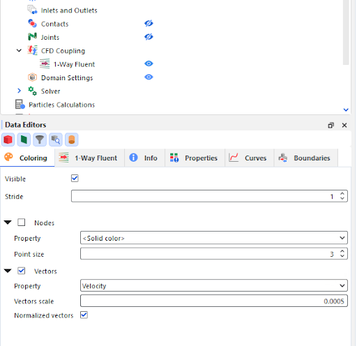
Figure 2.90: Vectors colored by the magnitude of the fluid velocity give insight to the flow field in 1-way coupled simulations.
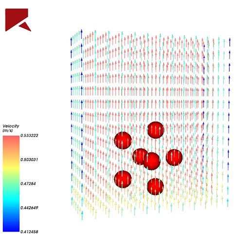
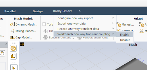
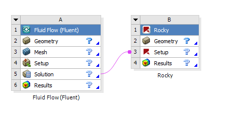
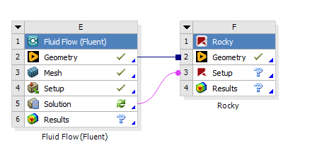
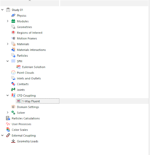
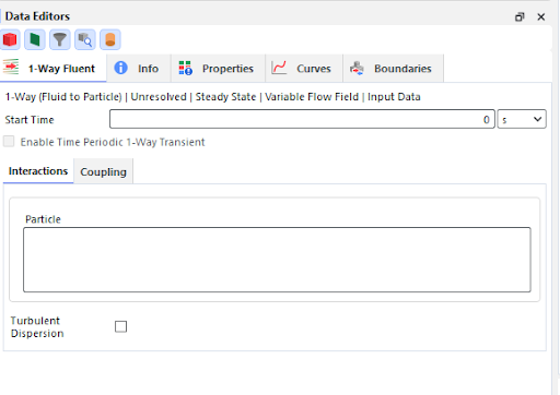
Drag the Fluent analysis onto the Project Schematic and set up the Fluent Project.
Important: You can only set up the 2-way coupled project if the Fluent Project is set up. Rocky looks for the .cas file for importing the necessary files for the 2-way coupling.
Drag a Rocky Analysis to the Project Schematics. Do not drop it on top of the Fluent setup.
Important: Do not drop it on top of the Fluent setup. The link must be created manually after both the two systems are placed at the Project Schematic.
Drag the Fluent Setup onto the Rocky Setup.
Select Unresolved as the 2-way coupling mode.
If the Fluent setup has Energy Model on, enable the Thermal in the Momentum tab of the Physics Data Editor in Rocky.`
When opening Rocky, the CFD Coupling entry at the Data Tree has the 2-Way Fluent mode selected.
Open the 2-Way Fluent data panel and edit the coupling setup as usual.
Figure 2.96: The Unresolved 2-way coupling mode is enabled, and the coupling setting can usually be edited.
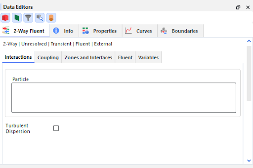
Set up the Fluent execution setting - select to run either in serial or parallel and the number of CPU processes that are used to solve CFD equations.
Important: As the Fluent run is controlled by Rocky in the 2-way coupling, the execution settings defined in the Rocky setup are used.
Figure 2.97: The Fluent tab allows the definition of the execution mode and the data used as the initial fluid field.
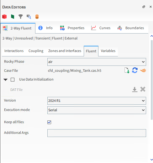
For prescribing an initial fluid field for the CFD solution, the .dat file should be imported at the Rocky setup.
Important: The current version does not allow the initial flow field to be imported from another Fluent run within the workbench. The fluent data file must be imported using the Fluent tab in Rocky.
For sharing the geometry between projects, link the Geometry of the Fluid project to the Setup of the Rocky project. Doing so, the geometry will be automatically imported into Rocky.
The CFD and DEM results of the unresolved 2-way coupling can be simultaneously post-processed in Rocky by opening the Setup entry of the Rocky project. Fluid quantities such as pressure and velocities can be analyzed and shown in the 3D view together with the particles.
The post-processing of additional fluid data can be done inside Fluent. For this purpose, a new Results component should be linked to the Fluent Solution of the coupled Rocky project.
Figure 2.100: The Fluent Solution entry should be used to send the fluid data for external post-processing.
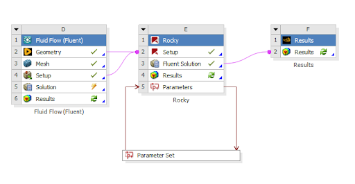
The Fluent Solution entry in the Rocky project should be used for sending the fluid data to another software, such as a post-processing software or a structural analysis.
For updating changes made to an upstream step, such as changes in a Fluent boundary condition or CFD mesh, select Refresh from the Rocky Setup entry.
Important: Any change in the Fluent Setup should be made in the Fluent Project that is linked to the Rocky simulation, not from the 2-way Fluent Data Editor in the Rocky UI. The reason is that the CFD setup from the Fluid Flow project will be copied and used as the base setup for the coupled simulation. Any changes made using Rocky will be overwritten when updating the workbench project.
Figure 2.102: If something is changed in an upstream component, the Refresh option in the Setup entry should be used to update the Fluent project used in the coupled simulation.
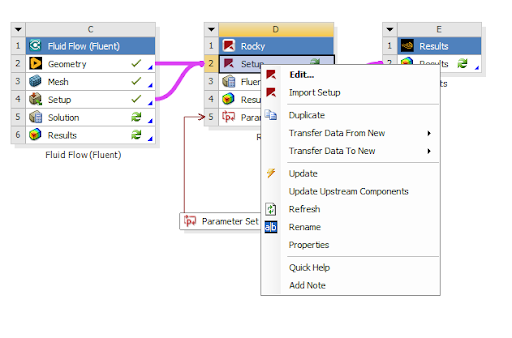
Inputs and Outputs parameters of the DEM simulation are exposed in the workbench as any other Ansys solver and can be used to evaluate several design points automatically.
Figure 2.103: The Fluent solution entry should be used for sharing the fluid data with another software, such as for structural analysis.
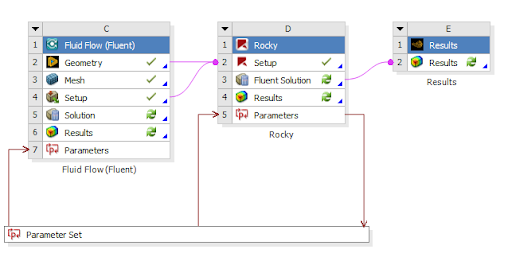
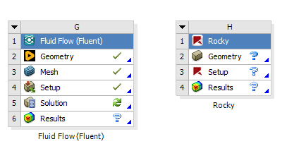
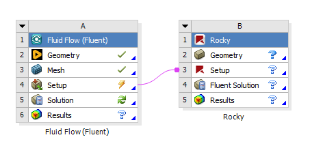
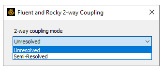
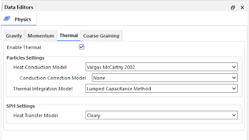
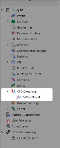
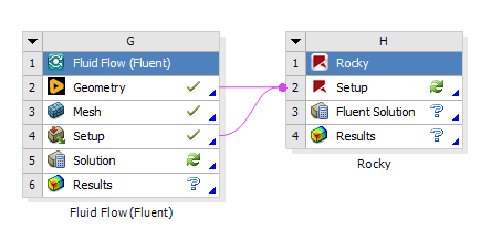
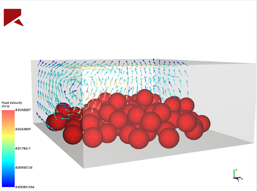
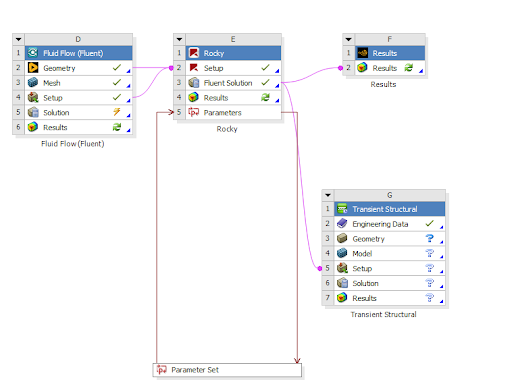
Drag the Fluent analysis and set up the Fluent Project.
Drag a Rocky Analysis to the Project Schematics. Do not drop it on top of the Fluent setup.
If the DEM simulation has no walls, you can Remove the Geometry Component.
Select Setup in the Rocky Project and click Edit. Select Semi-Resolved as the 2-way coupling mode.
When opening Rocky, the CFD Coupling entry at the Data Tree has the 2-Way Fluent Semi-Resolved mode selected.
In the 2-Way Fluent Semi-Resolved Data Editor, the coupling setup can be edited as usual.
For sharing the geometry between projects, link the geometry between the Fluid project and the Rocky Setup projects. Doing so, the geometry will be automatically imported into Rocky.
For the Semi-Resolved coupling, fluid data cannot be post-processed in Rocky. For post-processing fluid data, add a new Results component system and link it to the Rocky project Fluent Solution.
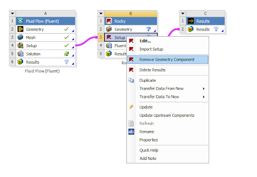
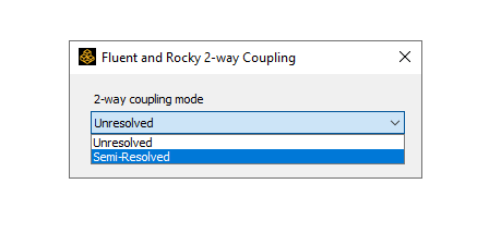
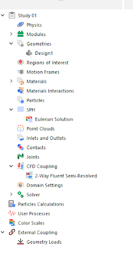
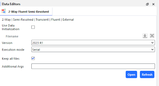
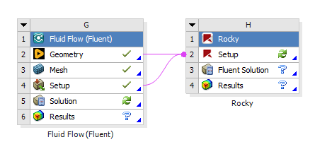
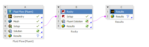
Workbench is integrated with Rocky through a special Addin. This is installed as a default component with your Rocky program (Figure 6).
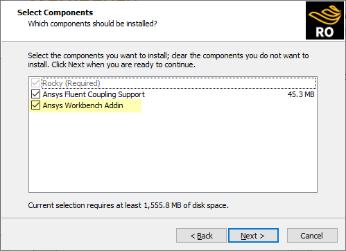
In addition, the Rocky installation will by default include all available versions of Ansys Workbench to integrate with the Addin (Figure 7). You must ensure that at least one version of Workbench is selected.
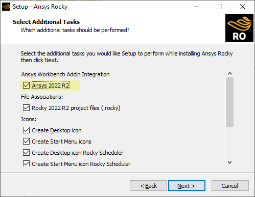
Beyond the above, there are no additional steps and no additional licenses required for you to begin using Rocky with Workbench.
Tip: See also the following topics:
After you have Ansys and Rocky installed on your computer, including the Rocky Addin explained above, you are ready to open Workbench and link it with Rocky.
Once you open Workbench and create a new Project, you can from the Toolbox panel, expand the Analysis Systems item, and then drag and drop Particle Dynamics (Rocky) to the Project Schematic (Figure 8). Note: This item will be referred to as the "Rocky" block for simplicity.
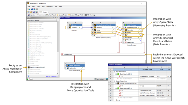
This creates a link between your Workbench project and the Rocky program. From here, you can either start a new Rocky project from within Workbench (Edit), or import a Rocky project into Workbench that you have already set up (Import Setup).
The link between your Workbench project and your Rocky project means that data will be automatically transferred between the two programs. In addition, it exposes Rocky input and output parameters, so you can explore Workbench capabilities such as evaluating multiple design points, creating Rocky cases automatically, and then running them through the weekend. (See also About Defining and Using Input Variables and About Defining Output Variables.)
The new Rocky Analysis System block (A) is made up of the components described in Figure 9.
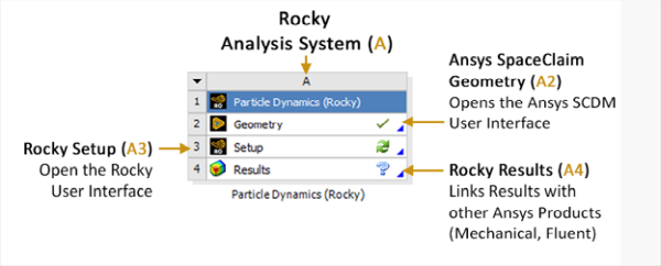
By interacting with the Rocky Analysis System block, and linking other items from the Workbench Analysis System-such as the Transient Structural block or the Static Structural block-to the Rocky items listed, you can have Workbench perform many different tasks in Rocky. This includes one-way coupled approaches with Ansys Mechanical, one-way coupled approaches with Ansys Fluent, standalone parametric studies, and more.
If you have linked to Rocky from within Workbench, an External Coupling entry will appear in the Rocky Data panel (Figure 10).
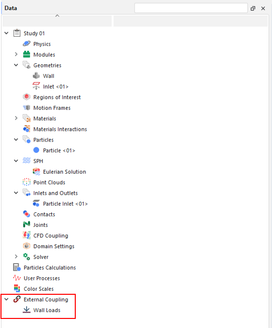
For Rocky projects opened through Workbench that are not coupled with Ansys Mechanical, this component will still appear in the Data panel but can be ignored.
To learn more about Workbench integration with Rocky, and to see Workbench in action, refer to the following resources:
See Also:
Rocky's integration with Ansys Mechanical enables Mechanical to conduct either transient or static structural analyses based upon the particle forces that Rocky calculates. These two tools can operate as connected components within Ansys Workbench, or the DEM portion can be done separately in Rocky and the results later imported into Workbench for the structural analysis portion.
Ansys Products needed: Ansys Rocky and Ansys Workbench
For projects coupled specifically with Ansys Mechanical, opening the Wall Loads in the Data Editors panel enables you to select which Rocky data items you want transferred to the Workbench connected Mechanical program.
For example, you can select which Walls you want to analyze in Mechanical, i.e, which loads are to be transferred and which load type you want between Force and Pressure.
See the image below:
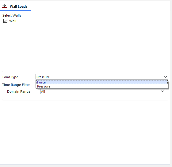
You can then select the results domain of the analysis that will be exported by setting the time range.
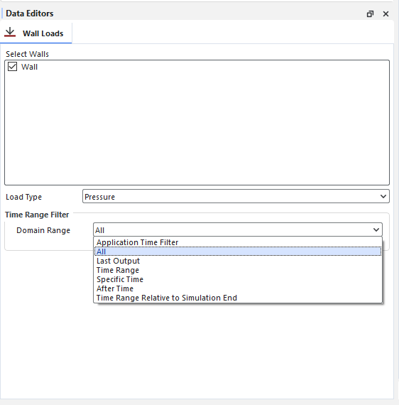
Important: When making a 1-way coupling with Mechanical (both 1-Way HTC and 1-Way Static and Transient Structural) the connection between Rocky Geometry and Results to Mechanical Geometry and Setup must be done manually, instead of dragging the Mechanical system and dropping it on top of the Rocky one. Otherwise, the coupling may not occur properly. This process is needed because now, for both 1-Way Static and Transient Structural (Forces only) and 1-Way HTC coupling between Rocky and Mechanical, the data from Rocky are automatically sent to Mechanical, and the manual process to copy and paste the .csv results inside Mechanical is no longer needed. For Pressure in the 1-Way Static and Transient Structural, the copy and paste is still needed.
Ansys Products needed: Ansys Rocky, Ansys Mechanical, Ansys Workbench, System Coupling and Ensight.
With this coupling is possible to send heat from Rocky and receive back the temperature from Mechanical using the System Coupling.
To do this, the users are able to create a coupled wall inside Rocky and the System Coupling will identify this walls as regions where the coupling is going to happen.
Limitations:
The coupled walls cannot have:
Motion Frame
Translation
Rotation
Mass tab
Wear tab
Replication tab
1- SETUP IN ANSYS ROCKY
Set up your simulation as you wish, then you will have to stipulate within Rocky which geometry of your simulation you want to couple.
To do this, right-click on the desired geometry, then click on Convert to and then on System Coupling Wall.
Click on File and then on Write System Coupling file. This step creates a file with information about where your Rocky file is for System Coupling.
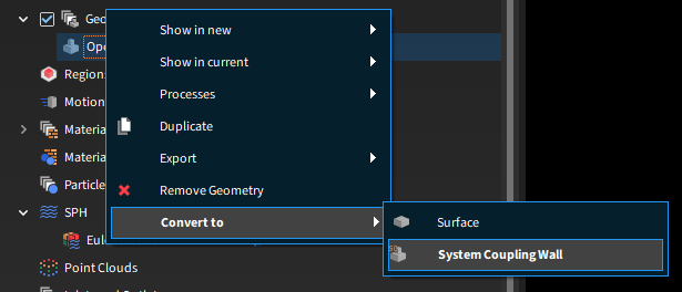

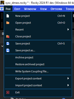

2- SETUP IN ANSYS MECHANICAL
Open your project in Ansys Mechanical and set the Initial Temperature and the System Coupling Region using the Transient Thermal option.
Set the System Coupling Region, as shown in the figures below:
Export the System Coupling File, by right-clicking on Transient Thermal and then on Write System Coupling Files.
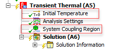
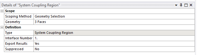
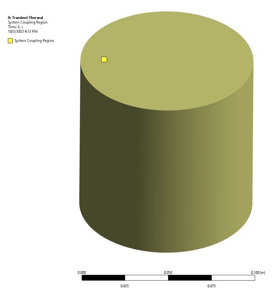
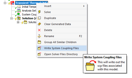
3- SETUP IN ANSYS WORKBENCH (TRANSIENT THERMAL)
Open your project in the Ansys Workbench and set the 2-way Thermal Coupling using the Transient Thermal option.
Learn more at About Rocky and Ansys Workbench Integration
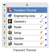
4- SETUP SYSTEM COUPLING
Open System Coupling and select a folder of your choice.
Tip: When you are doing this coupling, it is advisable to create three folders for your project, one for Rocky, another for Workbench and another for System Coupling.
Note: When add the folder some Warnings will appear in the message tag, but they will be resolved as you do the setup.
In the Data Panel, right-click Setup and then click Add Participant.
In the Add Participant window, select Input File and add the System Coupling File (.SCP) you saved from Rocky.
Repeat step 1, and in the Add Participant window, select Input File and add the System Coupling File (.SCP) you saved from Mechanical.
Your Data Panel must have both Rocky and Mechanical files:
In the Data Panel, right-click Setup and then click Add Coupling Interface.
Right Click on Coupling Interface and then click on Add Data Transfer.
Set the Data Transfer to Rocky as show in the figures below:
Repeat step 6, and set the Data Transfer to Mechanical as show in the figures below:
In the example below the Rocky Data Transfer is named as Temperature and the Mechanical Data Transfer is named as Heat Flow:
In Solution Control define the End Time and the Time Step Size.
Important: The same End Time and Time Step Size that you add in Rocky and Mechanical, you must add in System Coupling.
In Output Control, click on Results, and then on Type and select the Every Step option, as shown in the figure below:
Click on Start Solve.
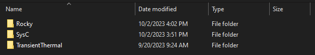
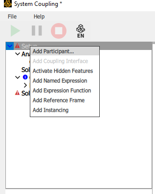
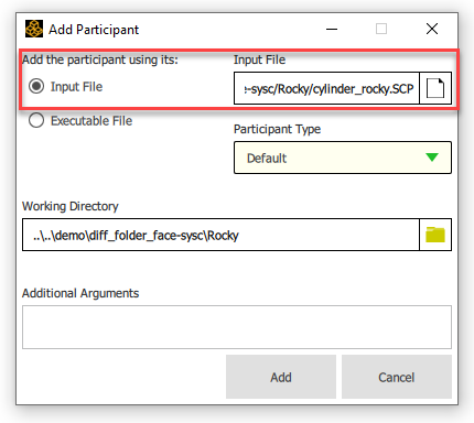
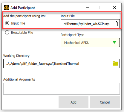
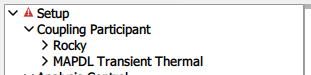
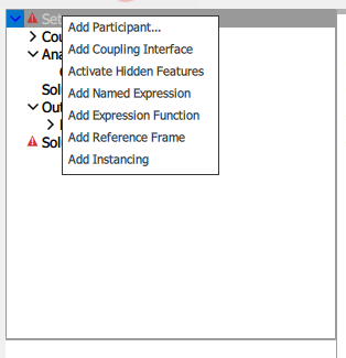
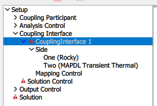
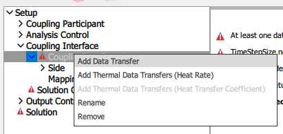
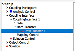
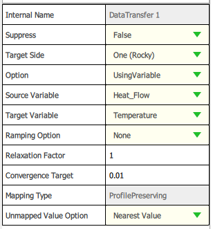
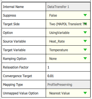
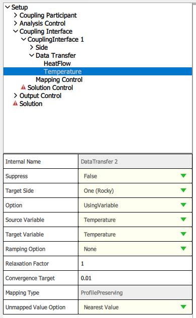
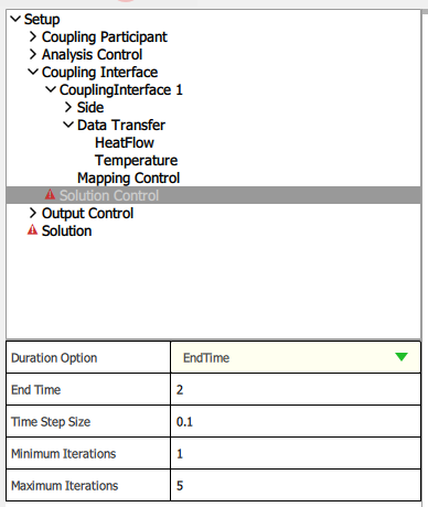
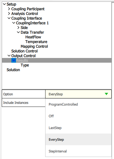
5- POST PROCESSING ENSIGHT
After solving your simulation, the post processing fase is carried out using the EnSight. Click on EnSight:
The geometries will appear in EnSight as shown in the figure below, one on top of the other, if you prefer you can separate them:
To see the results you have to drag the desired parameter to the geometry you want to see the result:
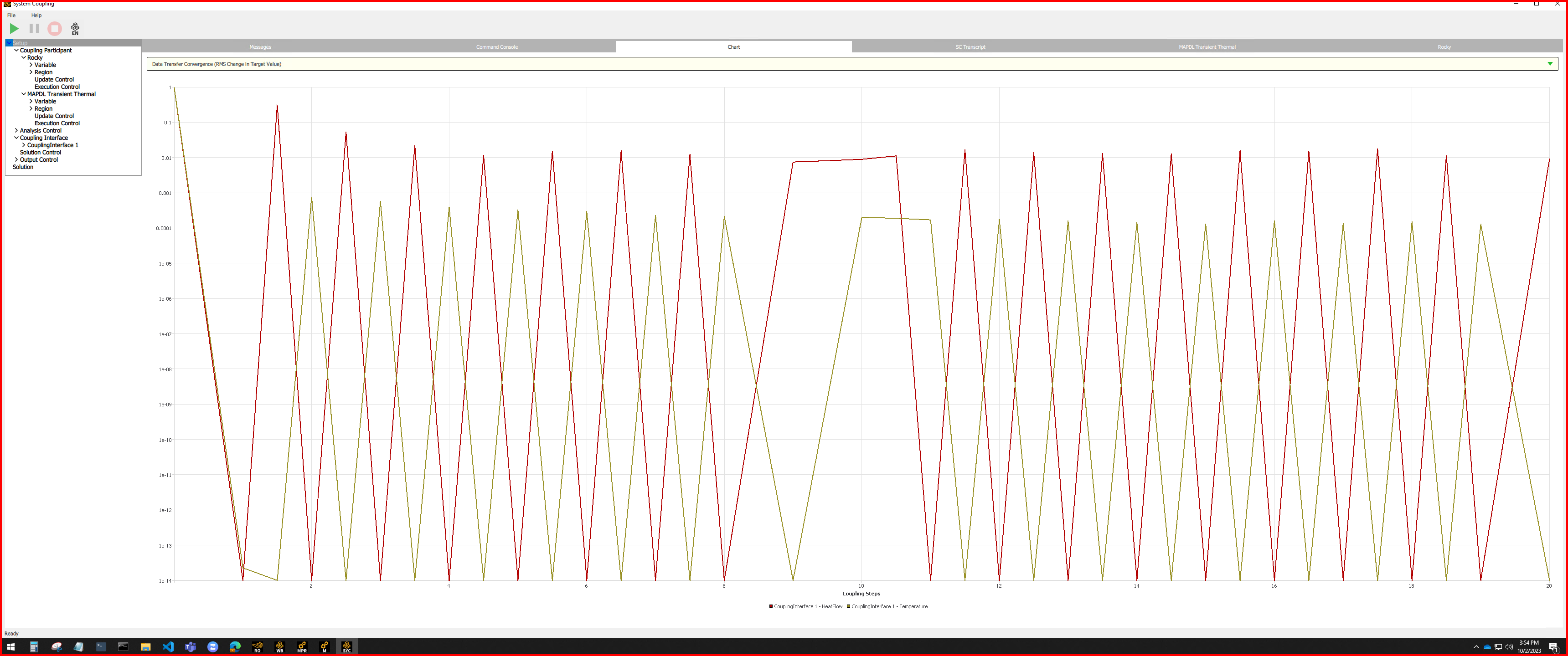
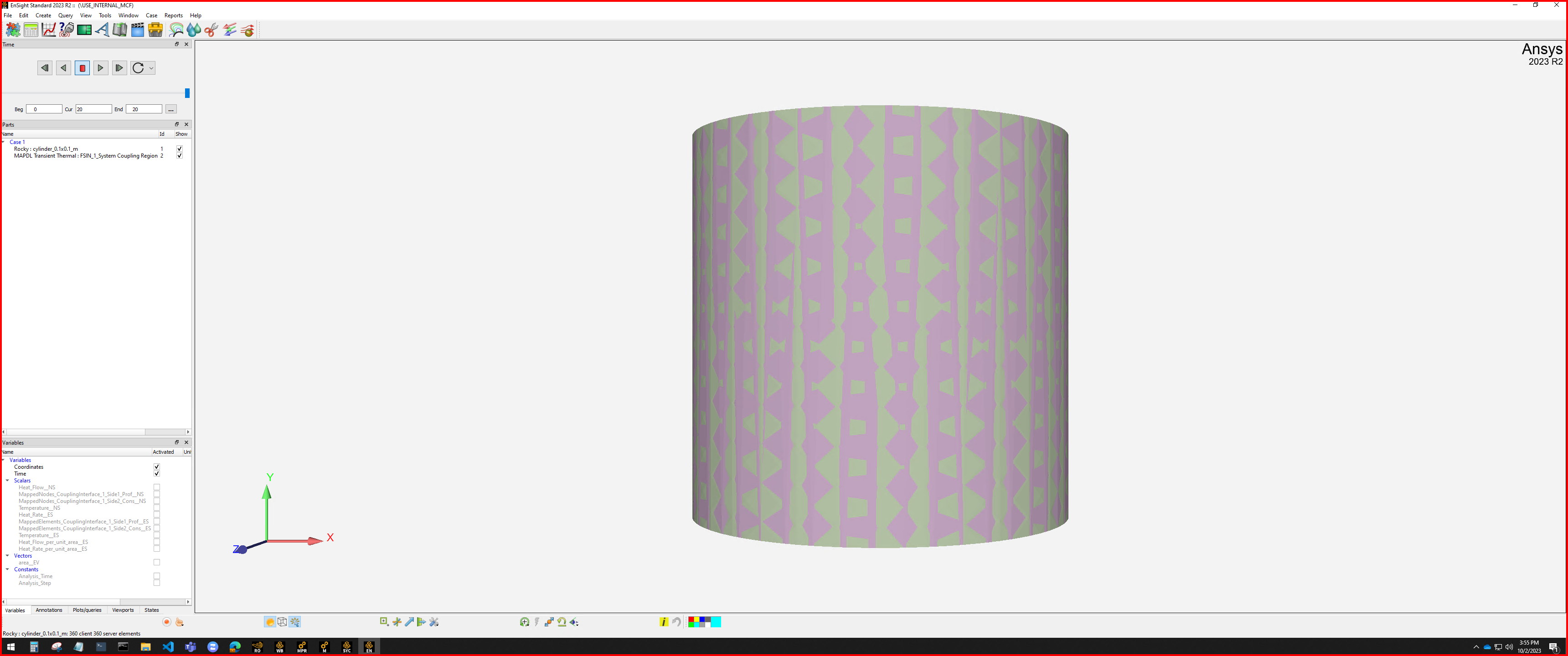
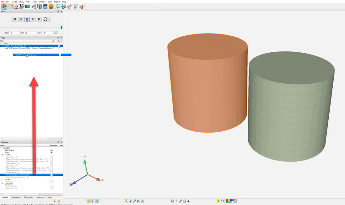
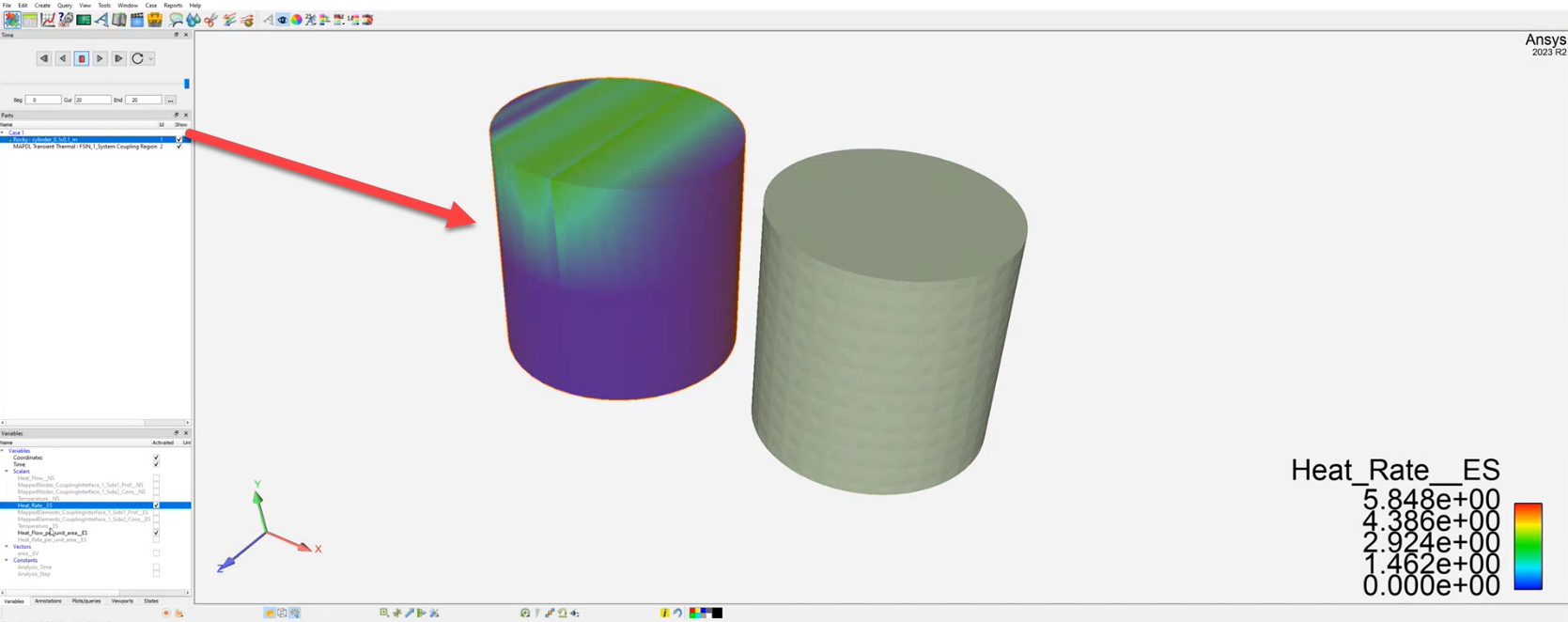
See Also:
Ansys Products needed: Ansys Rocky, Ansys Mechanical, Ansys Workbench, System Coupling and Ensight.
With this coupling, it is possible to send forces from Rocky and receive back the boundary displacement from Mechanical using the System Coupling.As the 2-Way Thermal coupling between Rocky and Mechanical (using the Transient Thermal one), the 2-Way Structural coupling uses the Transient Structural System inside Workbench. The main setup process is the same as already explained for the Thermal one, with just simple differences, that will be shown below.
1- SETUP IN ANSYS ROCKY
For the Rocky side, the first difference is that now, there are 2 Coupling Types options for the System Coupling Wall. For the 2-Way Structural Coupling, just select the Structural one. And for the 2-Way Thermal, just select the Thermal one.
The rest of Rocky setup, as well the Write System Coupling file is the same as 2-Way Thermal.
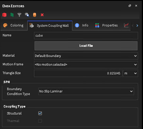
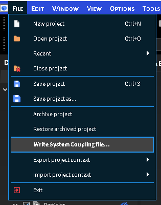
2- SETUP IN ANSYS MECHANICAL
The difference from the Mechanical side is that now, the Transient Structural system for the Workbench that will be needed, as show in this image
The Model data tree setup process follows the same default Structural one, with just the System coupling regions as already described for the Thermal.
One important point here is that the Time Step inside the Analysis System, for most of the cases, will need to have a small number, as the DEM-SPH collisions will happen in a small-time fraction, and as Mechanical is an Implicit Solver, the Time Step here will need to be smaller. With the biggest time steps, Mechanical will not be able to converge, and a High Element Distortion message will be shown in the System Coupling UI.
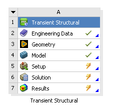


After the setup, the System Coupling Region must be exported.
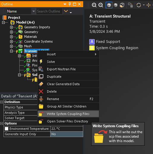
4- SETUP SYSTEM COUPLING
For the System Coupling side, all first steps are still the same. The only difference will be at Add Data Transfer, which now will have the Add FSI Data Transfer, which mainly will connect the forces data from Rocky, and send it to Mechanical.
Tip: When you are doing this coupling, it is advisable to create three folders for your project, one for Rocky, another for Workbench and another for System Coupling.
During the System Coupling solve process, it will be noticed that now, the Data Transfer will be the Force (Rocky to Mechanical) and Incremental Displacement (Mechanical to Rocky).
In the latest part, which is the post-processing, the two options remain: use Ensight directly from the System Coupling UI, or open Rocky and analyze the DEM-SPH trajectory and the Displacement results. At Ensight, new Variables are available, such as Force, Incremental Displacement, and Displacement Since Mesh Import, and for the Rocky side, the Displacement property will show up.
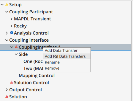
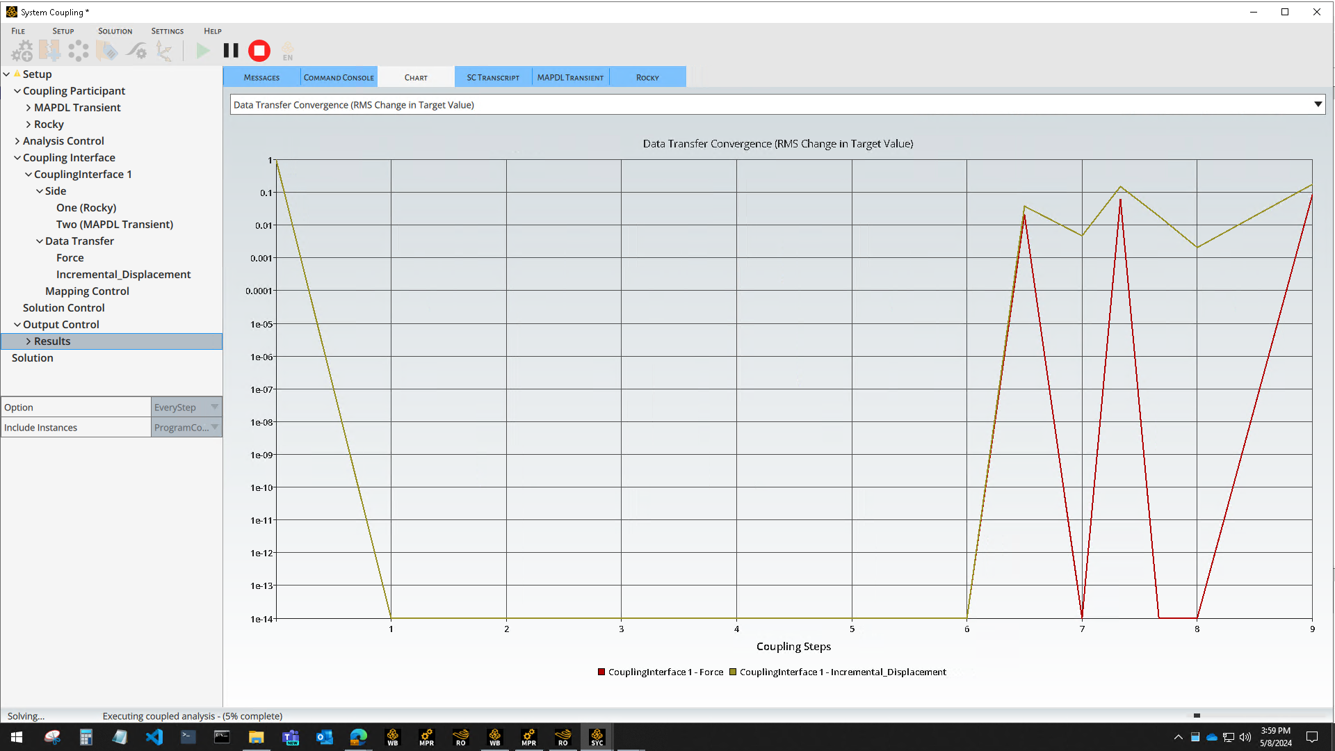
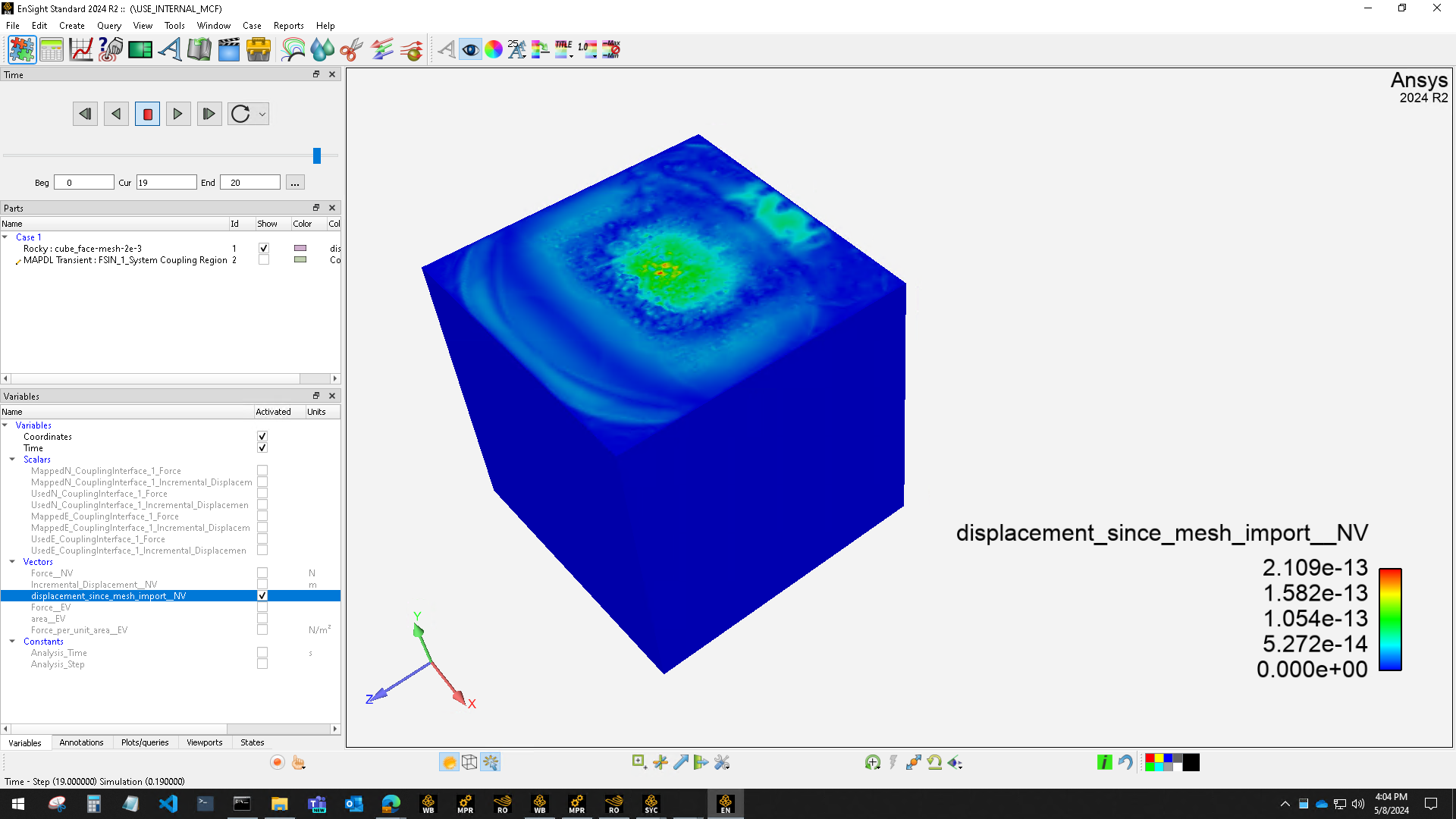
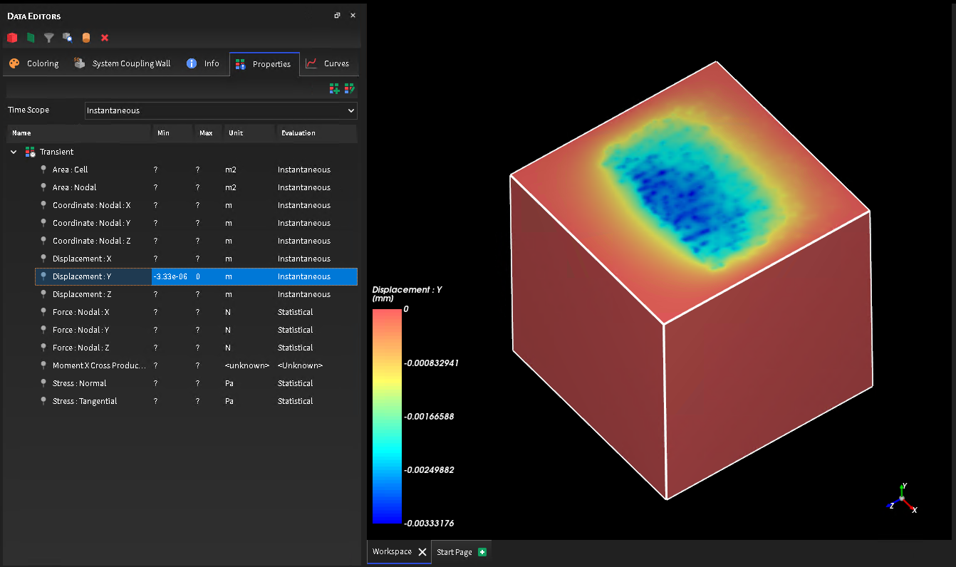
See Also:
Rocky's integration with Ansys Fluent in a 1-way coupled scenario enables Rocky to accept fluid flow and/or thermal property data from Fluent and then use that data to predict the resulting particle flow and/or related thermal properties. In a 2-way coupled scenario, Fluent and Rocky exchange fluid flow, particle forces, and thermal property data on a continual basis to discover how each interaction affects the other.
These two tools can operate as standalone products (for either 1-way or 2-way coupling) or can operate as connected components within Ansys Workbench (for 1-way coupling). But in order to make use of Fluent, an Ansys Coupling Component must be installed. (See also Install Ansys Coupling Components.)
Rocky 23R1 allows the computation of the heat transfer between particles and walls. For 2-way unresolved simulations, the heat exchange during collisions is transferred to the CFD solver and used to update the surface temperature. That way, the temperature of each boundary triangle is not predefined in Rocky, but is imported from the CFD solver at every time step.
For both 1-way and 2-way coupled simulations, the particle temperature is computed by Rocky accounting for the conductive heat transfer during collisions against walls and against other particles, as well as for the convective heat exchange with the fluid phase.
For 2-way coupled simulations, the boundary temperature changes are computed by the CFD solver accounting for the heat transferred to/from the fluid phase and the heat exchanged with the particles during particle-wall collisions.
For 1-way coupled simulations, the wall temperature changes according to the CFD solution exported to Rocky (and can vary spatially and in time), but the heat exchanged during particle-wall collisions is not transferred to the CFD solver.
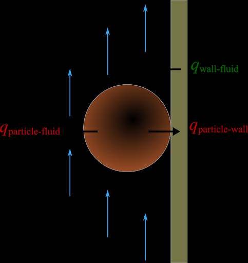
The coupled boundaries are automatically imported from the Fluent setup by selecting the desired walls from a list of compatible walls automatically populated in the CFD Coupling Boundaries tab.
These are the requirements for setting up a thermally coupled simulation.
The Rocky setup must have the Thermal model enabled.
The Fluent setup must have the Energy Equation turned on.
For 2-way coupled simulations, the walls must have Shell Conduction enabled in the Fluent setup, regardless of the Thermal Conditions option chosen.
Giving the wall thickness (thin wall model) but not turning on the shell conduction model does not make the wall compatible with the coupling.
Only walls in participating fluid domains can be thermally coupled to the DEM solution.
Mesh motion is not supported for thermally coupled boundaries.
Dynamic meshes (deforming meshes and remeshing) are not supported.
Polyhedral meshes are not supported.
To set up a Thermal Coupled Simulation, follow the steps below:
Import the Fluent case file and set up the required models listed in the Interactions, Coupling, Zones and Interfaces, Fluent and Variables tabs, as required for any 2-way coupled simulation.
Click the 2-Way Fluent entry in the Data Panel and navigate to the Boundaries tab in the Data Editors. Clicking on Load Fluent Boundaries will open a window listing all the compatible boundaries.
Tip: Check the Requirements entry to understand the compatibility criteria.
Select the walls you want to use for the thermal coupling.
For each selected wall, a new entry will appear under Geometries in the Data panel. These walls have specific icons as they are thermally coupled.
Unselecting the wall from the Load Fluent Boundaries list will remove the coupled wall from the Geometry list, as well as any user process linked to the coupled wall.
The coupled walls have fewer options compared to the standard walls as some models are not supported, such as wear and replication.
Select the Material to be assigned to the coupled wall.
Important: The mechanical properties of the assigned material will be used for computing contact forces for collisions between the particles and the wall, but the thermal properties required for the conductive heat transfer calculation will be extracted from Fluent.
Run the coupled simulation normally.
Two additional transient properties are available for coupled walls - Temperature and Thermal Conductivity. These triangle properties can be shown in 3D views or used to generate quantitative analyses such as time plots, histograms, or output parameters.
Figure 2.166: The wall temperature, initially at 300K, increases as hot particles (500K) collide with the wall.
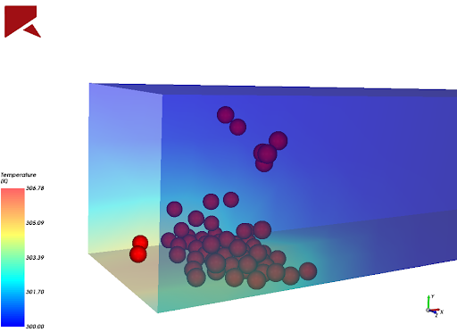
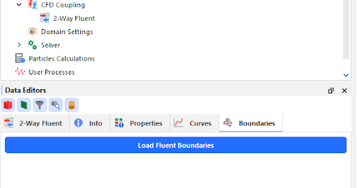
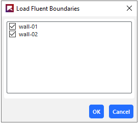
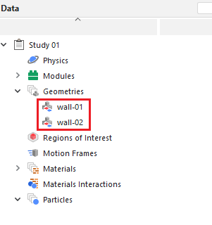
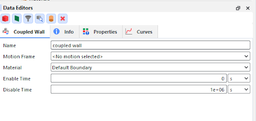
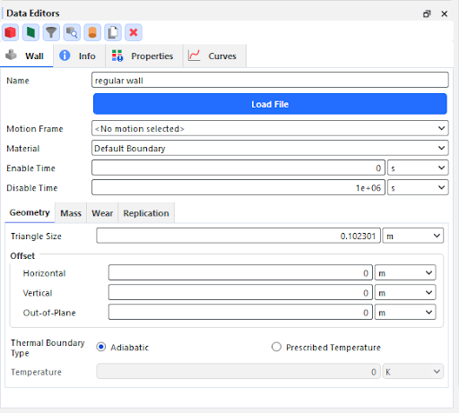
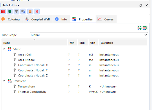
For setting up a 1-way thermal coupled simulation, there is only one additional step that must be completed. In the Rocky Export plugin, select Configure one-way export and then Select Wall Thermal Zones.
The Thermal Wall Selector window will list all the walls that are compatible with the 1-way thermal coupling between Rocky and Fluent.
Figure 2.168: List of all the walls compatible with the 1-way thermal coupling between Rocky and Fluent in the Thermal Wall Selector window.
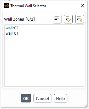
Pick the walls that you wish to participate as coupled walls.
Run the simulation normally and export the results to Rocky using the Rocky Export Plugin.
In Rocky, enable Thermal and select Fluent (Fluid -> Particle) as the coupling mode.
Select the F2R file that was exported from Fluent. Set up the required models listed in the Interactions and Coupling tabs, as required for any 1-way coupled simulation.
Click the 1-way Fluent entry in the Data Panel and navigate to the Boundaries tab in the Data Editors.
Clicking on Load Fluent Boundaries will open another window listing all the compatible boundaries. Tip: Check the Requirements entry to understand the compatibility criteria.
Select the walls you want to use for the thermal coupling.
For each selected wall, a new entry will appear under Geometries in the Data panel. These walls have specific icons as they are thermally coupled.
Unselecting the wall from the Load Fluent Boundaries list will remove the coupled wall from the Geometry list, as well as any user process linked to the coupled wall.
The coupled walls have fewer options compared to the standard walls as some models are not supported, such as wear and replication.
Select the Material to be assigned to the coupled wall.
Important: The mechanical properties of the assigned material will be used for computing contact forces for collisions between the particles and the wall, but the thermal properties required for the conductive heat transfer calculation will be extracted from Fluent.
Run the coupled simulation normally.
Additional properties are created for the coupled walls. These can be used for quantitative analyses, such as time plots and histograms, for creating output parameters or for coloring the wall triangles in a 3D view.
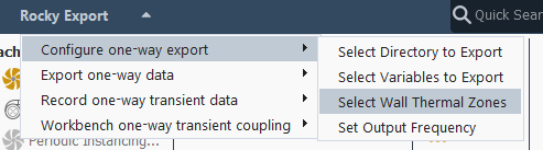
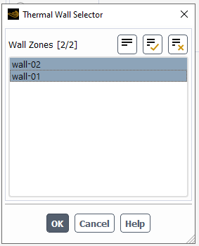
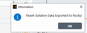
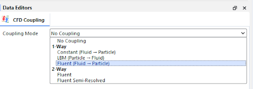
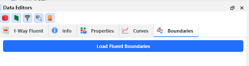
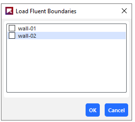

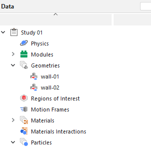
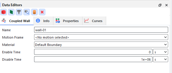
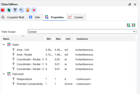
The ways in which Rocky and Ansys Fluent can work together are covered in the following topics:
See Also:
In this version of Rocky, coupling with Ansys Motion is done through an external module. Refer to the Ansys Motion Coupling information on the Ansys Learning Hub for more information: https://jam8.sapjam.com/blogs/show/oPXtQy8gStuFJpHirxTRNK.
See Also:
For more information about Rocky integration with Ansys optiSLang, refer to the information on the Ansys Learning Hub: https://jam8.sapjam.com/wiki/show/b4PtFm5qN24UE6HWBfgyTU.
See Also:
For more information about Rocky integration with Ansys Minerva, refer to the information on the Ansys Learning Hub: https://jam8.sapjam.com/wiki/show/cEdhCVNehj2TLx3sWJGmES.
See Also:
In Rocky, Modules refer to separate pieces of code that when explicitly turned on (or enabled) prior to processing your simulation, add in discrete features or functionality within your project.
There are several types of Modules, several ways you can gain access to Modules, and several ways in which Modules can affect your simulation setup and post-processing.
What would you like to do?
Learn more About Rocky Modules
Learn more about Rocky Simulation Entities that can be Affected by Modules
See Also:
In Rocky, Modules refer to separate pieces of code that when explicitly turned on (or enabled) prior to processing your simulation, add in discrete features or functionality within your project. This enables you to include-or even develop yourself-custom or specialized functionality into your Rocky projects without having to acquire a new version of the Rocky product itself.
There are several ways in which you can acquire Modules, and several ways Module functionality can affect how you set up your Rocky projects. See below sections for details.
In this version of Rocky, several features are provided via Modules, including Collision and Particle Statistics. Because these Modules are provided by default with your Rocky installation, these are sometimes referred to as embedded Modules.
Conversely, you may also have access to external Modules, which are custom Modules installed separately from the Rocky product.
The embedded Modules included by default with Rocky (Figure 1) include the following:
Boundary Collision Statistics. which enables the collection of boundary-related collision data, such as collision frequency, intensities, and impact velocities.
CFD Coupling Particle Statistics, which enables the collection of fluid-particle interaction data.
Contact Energy Spectra, which enables the collection of collision-based energy values during the simulation and the resulting data is categorized by the contact pair (particle group and/or geometry).
Contacts Overlap Monitor, which checks each contact pair (particle-particle or particle-boundary) for the amount that they overlapped-the percentage of which is determined by the size of the smallest particle in the contact pair-and raises a message in the Simulation Log panel if an overlap exceeds any of the three warning levels you define.
Inter-group Collision Statistics, which enables the collection of energy dissipation data for each particle-particle and particle-boundary pair.
Inter-particle Collision Statistics, which enables the collection of particle-related collision data between all particles in the simulation.
Intra-particle Collision Statistics, which enables the particle-related collision data affecting the surfaces of a particular particle set.
Joint Statistics, which enables the collection of joint-related statistical data.
Particle Instantaneous Energies, which enables the calculation of the kinetic and potential energies of each individual particle in the simulation. These energies are useful when performing global or partial energy balances in a simulation.
Particles Energy Spectra, which enables the collection of energy values during the simulation that are related only to particles, and the resulting data is classified by size and particle group.
SPH Boundary Interaction Statistics, which enables SPH boundary-related data, generating properties of the forces that the fluid is exerting on the walls. Also, curves may be generated for the resultant forces, torques and power.
SPH Density Monitor, which enables the monitoring of density values of the
SPH HTC Calculator, which calculates the heat transfer coefficient (HTC) through forced convection for each wall triangle.
SPH elements during a simulation. - SPH Mass Flow Rate, which enables to measure the mass flow rate in the chosen surface.

Because these Modules are included with the Rocky product, they will be documented as usual in the User and Technical Manuals.
You may have access to other external Modules not included by default in Rocky. These might have been custom Modules created by you using the Rocky Software Development Kit (SDK), separate functionality provided to you through the Ansys Learning Hub (see the API:Solver - Functional Modules page here: https://help.esss.co/ansysrocky-modules/), or shared with you by others.
Tips: To learn more about making your own custom Modules, do one or more of the following:
Access the Rocky API:Solver Manual. (From the Help menu, point to Manuals, and then click API:Solver Manual.)
External Modules are typically installed via ZIP file (see also Install an External Module). After installation, they will appear in Rocky under Modules in the Data panel.
Because these Modules are installed separately from the Rocky product, their documentation (if available) will be separate, too.
Tip: You will know if an external Module has included documentation if you see an Open this Module's Help File icon (?) on the Module's main tab in the Data Editors panel. Clicking this icon should open the Module's documentation in a separate window.
What would you like to do?
Learn more about Rocky Simulation Entities that can be Affected by Modules
Learn more About Modules Parameters
See Also:
Once you enable a Module (see also About Modules Parameters), there can be other places in the Rocky UI affected by that particular Module. How and what *simulation entities* can be affected depends upon the Module and how it was built.
Typically, enabling a Module can affect the Rocky UI in one or more of the following ways:
The Module overrides Rocky's default models or settings. Models or settings that can be overwritten by a Module are considered to be exclusive. An exclusive model or setting allows a Module to disable its default options and replace them with the name of the Module.
The Module adds additional models or settings. Models or settings that are added to the Rocky UI as a result of enabling a Module are considered to be non-exclusive. A non-exclusive model or setting allows a Module to add new options to its default set of options, but does not allow the Module to override any default options.
See the below sections for more detail about each of these two Module-related UI conditions. In addition, refer to Table 1 below to learn what areas of the Rocky UI might be affected by a Module.
Rocky UI settings that are considered to be exclusive have the effect of disabling Rocky's default options for a particular model or setting, and then replacing them with the name of the Module. In these cases, you must use the model or setting defined in the enabled Module, and only one enabled Module can override any particular model or setting at one time. This means that if you happen to have more than one Module defining the same exclusive model or setting in different ways, you must enable only one of those Modules in your simulation setup.
Rocky UI settings that are considered to be non-exclusive have the effect of adding in additional models or settings for the Module, but do not override any default models or settings. Sometimes the additional models or settings appear on a separate Modules tab within the affected simulation entity, and sometimes new options are added to existing entities or lists.
No matter how these appear to you in the UI, if you have enabled a Module that includes additional models or settings, you must make use of those Module-related models or settings at least once in your simulation setup. This means that, for example, if you have two enabled Modules that define the same non-exclusive model for individual Particle sets in two different ways, you must define at least two different Particle sets to make use of the two different models that were added by their respective Modules.
The table below lists the areas of the Rocky UI that are able to have their settings and options modified by a Module that is enabled.
Tip: Refer to the Module's documentation for further details about Module-specific parameters. Specifically:
For embedded Modules, this documentation can be found in the Rocky User Manual (the document you are reading now).
For external Modules, this documentation (if provided) can be found by clicking the Open this Module's Help File icon (?) on the Module's main tab in the Data Editors panel.
Table 1: Simulation Entities that can be affected by Modules, and how they can be affected
Simulation Entity | Setting or Area Affected | How Affected | See Also |
|---|---|---|---|
Physics | Momentum tab | Normal Force; Tangential Force; Adhesive Force; Impact Energy | Built-in model override (exclusive settings) | |
Physics | Thermal tab | Heat Conduction Model; Thermal Integration Model | Built-in model override (exclusive settings) | |
Individual imported Geometries | New Modules sub-tab | Additional settings added | |
Individual imported Geometries | Wear | Wear Law | Additional models added (non-exclusive settings) | |
Individual Feed Conveyor Geometries | New Modules sub-tab | Additional settings added | About Feed Conveyor Parameters |
Individual Receiving Conveyor Geometries | New Modules sub-tab | Additional settings added | About Receiving Conveyor Parameters |
Individual Materials | For each Material defined under Materials, a new group box labeled with the Module's name | Additional settings added | |
Materials Interactions | For each pair of materials interactions, a new group box labeled with the Module's name | Additional settings added | |
Individual Particle set | Composition | Joint Model; Breakage | Model; Breakage| Fragment distribution | Distribution model | Additional models added (non-exclusive settings) | |
Individual Particle set | New Modules sub-tab | Additional settings added | |
Inputs | New Modules sub-tab | Additional settings added | |
CFD Coupling | 1-Way Fluent tab; CFD Coupling | 2-Way Fluent tab; CFD Coupling | 1-Way Constant tab | Interactions | Drag Law; Interactions | Lift Law; Interactions | Torque Law; Interactions | Virtual Mass Law; Interactions | Convective Heat Transfer Law | Additional models added (non-exclusive settings) | About Using the 1-Way Fluent Method; About Using the 2-Way Fluent Method; About Using the 1-Way Constant Method |
See Also:
In this version of Rocky, many more additional models and functionality are available as external Modules that can be downloaded from the Customer Portal.
Note: Even though this install procedure is similar on both Windows and Linux machines, be aware that Module ZIP files are specific to both the operating system and the version of Rocky for which the Module was created.
Locate or download the ZIP file for the external Module you want to install. Tips:
Many external modules created by ESSS can be downloaded from the Customer Portal on the API:Solver - Functional Modules page: https://help.esss.co/ansysrocky-modules/.
Ensure that the ZIP file you download is appropriate for both the operating system and the Rocky version you are using.
Note: The Ansys Motion Coupling module has its own unique installation steps and requirements. Refer to the installation page here https://jam8.sapjam.com/blogs/show/oPXtQy8gStuFJpHirxTRNK for instructions. (See also About Rocky and Ansys Motion Integration.)
Into your user folder's
..RockyModulesfolder, extract the contents of the ZIP file. For example:In Windows, this might be your
%USERPROFILE%DocumentsRockyModulesfolder.In Linux, this might be your
~/.Rocky/Modulesfolder.
Once extracted, the ZIP file will automatically create a build folder in the
Modulesfolder and the Module contents will be installed there.If the Rocky program is open, close it and open it again to refresh the Modules list. The external Module should be listed in the Modules entity. (From the Data panel, select Modules and then from the Data Editors panel, review the Modules list.)
See Also:
There are several parameters you can set in Rocky that will affect your overall simulation. These include various preferences and unit types, as well as variables and scripts. These items can be determined before you set up your simulation, or can be modified at any point during the setup process.
What would you like to learn about?
See Also:
Global preferences for Rocky include settings like memory usage, date and time format, video, plot and view options. What you choose to set in preferences will affect the rest of the Rocky user interface.
What would you like to do?
When you set your global preferences, you determine what global (default) options you want to set for memory usage, date format, timestep format, drag and drop, Internet proxy, video encoding and quality, and display for Rocky windows, including 3D Views, plots, and histograms. You can also view (but not edit) what keyboard shortcuts perform which commands.
The settings that you choose in the Preferences dialog will persist throughout your entire Rocky experience. Some settings, like memory usage and Internet proxy settings, can only be changed from the Preferences dialog. Other settings, like window displays, affect only what default settings appear in the various panels within the Rocky UI but can be overridden from the panel whenever you want.
Important: Changes you make within the Preferences dialog may not immediately affect in-process features or functionality. To ensure that all changes you make within this dialog are applied immediately, click OK on the Preferences dialog, and then close and reopen any Rocky windows, panels, or projects affected by the Preferences changes you made.
See the images and table below to help you understand what to set for your global preferences on properties not including those on the Windows panel.
The Properties settings listed under Windows on the Preferences dialog affect only the configuration used to create windows of the selected type. Any of these default settings can be overridden from the Window Editors panel whenever you want.
See the images and tables below to help you understand what global preferences to set for Windows panel-related items.
Also, see additional information on these settings in the following topics:
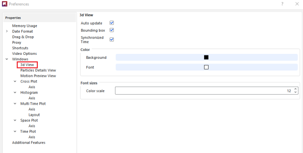
Table 2: Preferences options for 3d View Windows
Property | Description | Range |
|---|---|---|
Auto update | When enabled, any change made to the display settings of the selected 3D View or to the items affecting the data or settings calculated and displayed within the 3D View, including the output time or Properties displayed, will be updated in the 3D View automatically. Because automatically updating the view with each separate change can be computationally intensive, you can clear this option to have all calculated items and more computationally intensive display options remain unchanged in the 3D View until you enable Auto update again. Tip: You will know when the calculations in a 3D View window are not being updated when you see a thick red border around the window. | Turns on or off |
Bounding box | When enabled, displays measurements illustrating the simulation entity in the selected 3D View. | Turns on or off |
Synchronized Time | When enabled and the window (or any other window with this checkbox enabled) is selected, the details shown in this (and any other Synchronized Time) window will be updated when the current output time is changed on the Time toolbar. (See also About the Time Toolbar.) When cleared and the window is selected, only this window will be updated when the current output time is changed on the Time toolbar. Tip: To keep the output time synchronized between multiple 3D View or other windows, ensure each window has this option enabled. | Turns on or off |
Color Background | Enables you to change the color that appears behind the geometries and particles in the 3D View. | Options limited by the choices in the Select Color dialog |
Color Font | Enables you to change the color of the labels, borders, and axes lines displayed in the 3D View. Note: These color options can be overridden for text overlays by using the Color option on the Overlays tab. (See Table 3 below.) | Options limited by the choices in the Select Color dialog |
Font sizes Color scale | Enables you to change the size of the text used on color scales for Properties, which, unlike the other lines or labels displayed on the 3D View, is not affected by the window size or the level of zoom you have applied. | Whole values from 1 to 100 |
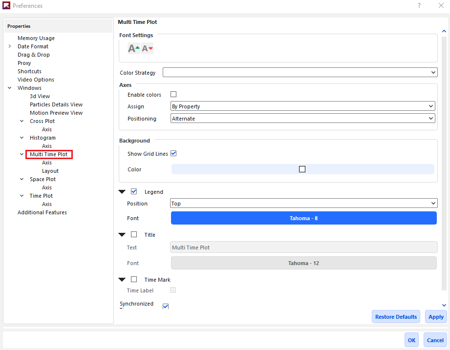
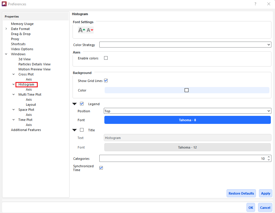
Table 3: Preferences options for Graph (Plot and Histogram) Windows
Setting | Description | Range |
|---|---|---|
Font Settings | The following two buttons in this section apply to all axes, legend, and title text shown in the graph:
Notes:
|
Increase font size; Reduce font size |
Color Strategy | Changes the coloring criteria of the curves, which affects the legend text and plot line of the properties (Property or Curves) being graphed. This option can be used to group curves with a similar representation by color based upon the following options:
| Entity Based; Property Based; Unique |
Axes Enable colors | Enabling this checkbox colors the Y axes according to the Color Strategy selected. Clearing this checkbox keeps all axes colored black. | Turns on or off |
Axes Assign | For plots with multiple Properties or Curves, this enables the Y axes to be shared according to the following options:
| By Quantity; By Property |
Axes Positioning | For plots only, this sets on which side of the graph the axes will be displayed. Specifically:
| Alternate; Left Axes First; Right Axes First |
Background Show Grid Lines | Selecting this checkbox enables black grid lines to appear behind your graph. | Turns on or off |
Background Color | Enables you to choose the color that appears behind your graph. | Options limited by the Select Color dialog |
Legend | Enables the legend information, the content and color of which are determined by the Color Strategy setting, to be displayed on the graph window. | Turns on or off |
Legend Position | When Legend is enabled, determines where the Legend information appears on your graph. | Bottom; Left; Right; Top |
Legend Font | Enables you to change the type, style, size, and effects of the font used for displaying the Legend text. Note: The size you choose will still be affected by the Font Settings buttons. | Options limited by the Select Font dialog |
Time Mark | For Time and Multi Time Plots only, enables a dotted, vertical line to be displayed at the location of the current output time. | Turns on or off |
Time Label | When Time Mark is selected, enables you to add a label to the mark displaying the current output time value. Note: The value displayed reflects the units used for the Time (X) axis. | Turns on or off |
Title | Enables you to add a separate title to the top of the graph. | Turns on or off |
Title Text | When Title is selected, determines what text will be displayed in the title. | No limit |
Title Font | Enables you to change the type, style, size, and effects of the font used for displaying the Title text. Note: The size you choose will still be affected by the Font Settings buttons. | Options limited by the Select Font dialog |
Categories (same as Number of Bins elsewhere) | For histograms only, enables you to choose the number of bins or bars the data is aggregated into. | Whole numbers greater than 1 |
Synchronized Time | When enabled and the plot window (or any other window with this checkbox enabled) is selected, the details shown in this (and any other Synchronized Time) window will be updated when the current output time is changed on the Time toolbar. (See also About the Time Toolbar.) When cleared and the window is selected, only this window will be updated when the current output time is changed on the Time toolbar. Tip: To keep the output time synchronized between multiple plot or other display windows, ensure each window has this option enabled. | Turns on or off |
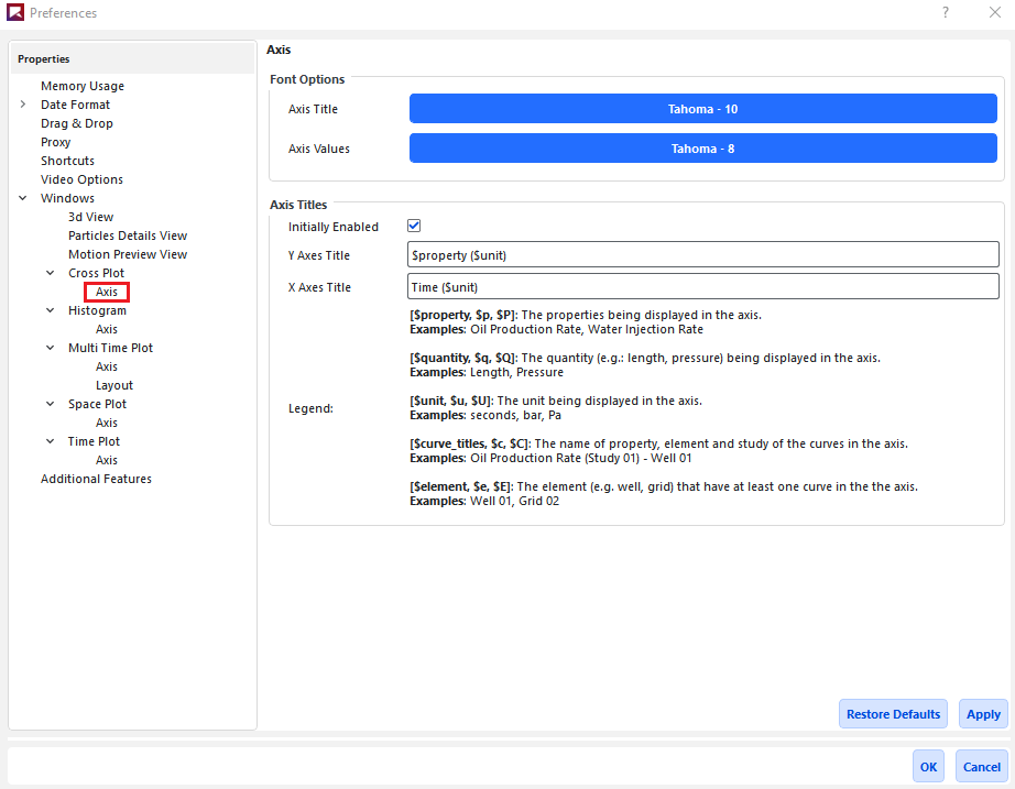
Table 4: Preferences options for Axes on Graph (Plot and Histogram) Windows
Setting | Description | Range |
|---|---|---|
Font Options | ||
Axis Title | Enables you to change the type, style, size, and effects of the font used for displaying the title Text for the selected axis. Note: The size you choose will still be affected by the Font Settings buttons located on the first tab of the Window Editors panel. | Options limited by the Select Font dialog |
Axis Values | Enables you to change the type, style, size, and effects of the font used for displaying the value marks for the selected axis. Note: The size you choose will still be affected by the Font Settings buttons located on the first tab of the Window Editors panel. | Options limited by the Select Font dialog |
Axis Titles | ||
Initially Enabled | When selected, default axis titles will be added to the plot. When cleared, no axis titles will appear by default; you must manually turn on Axis Title from the Window Editors panel when you want an axis title to show. | Turns on or off |
Y Axes Title | Enables you to specify the default format for titles appearing on the Y axis. Any Keywords you specify will be replaced with the corresponding data in the Axes Title field, and will be updated when the data supporting the Keyword changes. Tip: Sample Keywords are provided in the Legend section. | No limit |
X Axes Title | Enables you to specify the default format for titles appearing on the X axis. Any Keywords you specify will be replaced with the corresponding data in the Axes Title field, and will be updated when the data supporting the Keyword changes. Tip: Sample Keywords are provided in the Legend section. | No limit |
Legend | Displays sample Keywords you can use when defining Axes Title information. | Display only |
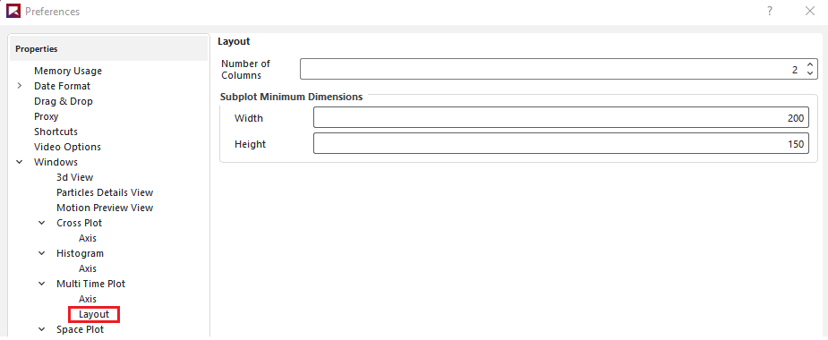
Table 5: Preferences options for Layout on Multi Time Plot Windows
Setting | Description | Range |
|---|---|---|
Number of Columns | Enables you to set how many columns into which you want the sub-plots of your selected Multi Time Plot arranged. | Whole numbers greater than or equal to one |
Subplot Minimum Dimensions Width | Enables you to define the minimum pixel width you want Rocky to maintain for each individual sub-plot in the selected Multi Time Plot. When making the window size smaller, the sub-plots will continue to be displayed in full until this setting is reached, at which point scroll bars will be added. | Whole values greater than or equal to 300 |
Subplot Minimum Dimensions Height | Enables you to define the minimum pixel height you want Rocky to maintain for each individual sub-plot in the selected Multi Time Plot. When making the window size smaller, the sub-plots will continue to be displayed in full until this setting is reached, at which point scroll bars will be added. | Whole values greater than or equal to 150 |
What do you want to do?
See Also:
From the Options menu, click Preferences.
From the Preferences dialog, choose the category you want under Properties, and then make the choices you want on the right. Note: Shortcuts are not currently editable.
Click Apply to save your changes.
Repeat steps 2-3 until you have set all the options you want, and then click OK to close the dialog. Tip: To ensure that all changes you made within this dialog are applied immediately, close and reopen any Rocky windows, panels, or projects affected by the Preferences changes you made.
See Also:
Before you begin using Rocky, it is important that you understand the units used in the user interface and set them the way you want.
What would you like to do?
See Also:
Currently, there are two unit systems included in Rocky: the International System and the English. You can choose to use one of these two included systems, or you can create your own custom unit system.
Whatever system you choose will provide the default unit settings for all parameters used within Rocky. However, each individual parameter unit can still be changed manually to another unit type at any time.
Use the images and tables below to help you understand your unit system options.
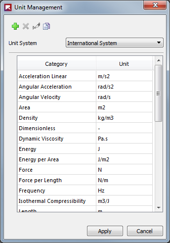 Figure 1 : Unit Management dialog
Table 1: Unit Management dialog options
Setting | Description | Range |
|---|---|---|
Unit System | Sets the unit system used by default throughout Rocky. Choices include:
If you have created custom unit systems, those will display in this list also. | Lists all default and custom unit systems for Rocky. |
Category | Lists the descriptive name of the item being measured. | Automatic |
Unit | Provides the unit symbol that will be used by default for the parameters in Rocky. These are editable when you choose to create a custom system. | Automatic |
Table 2: Default Units Used in Rocky
Item | International Unit | International Unit Symbol | English Unit | English Unit Symbol |
|---|---|---|---|---|
Acceleration Linear | meter per second squared | m/s2 | foot per second squared | ft/s2 |
Angular Acceleration | radian per second squared | rad/s2 | radian per second squared | rad/s2 |
Angular Velocity | radian per second | rad/s | radian per second | rad/s |
Area | square meter | m2 | square foot | ft2 |
Density | kilogram per cubic meter | kg/m3 | pound mass per cubic foot | lbm /ft3 |
Dimensionless | - | - | - | - |
Dynamic Viscosity | Pascal second | Pa⋅s | centipoise | cP |
Energy | joule | J | foot pound force | ft⋅ lbf |
Energy per Area | joule per meter squared | J/m 2 | pound force per foot | lbf /ft |
Force | Newton | N | pound force | lbf |
Force per Length | Newton per meter | N/m | pound force per foot | lbf /ft |
Frequency | hertz | Hz | hertz | Hz |
Isothermal Compressibility | cubic meter per joule | m3/J | cubic meter per joule | m3/J |
Kinematic Viscosity | square meter per second | m2/s | centistoke | cSt |
Length | meter | m | foot | ft |
Mass | kilogram | kg | pound mass | lbm |
Mass Flow Rate (formerly "Tonnage") | metric tons per hour | t/h | pound mass per hour | lbm /h |
Mass per Energy | kilogram per joule | kg/J | pound mass per foot pound force | lbm / ft⋅lbf |
Moment of Force (formerly "Torque") | Newton meter | N⋅m | foot pound force | ft⋅lbf |
Moment of Inertia | kilogram meter squared | kg⋅m2 | square foot pound mass | lbm⋅ ft2 |
Percentage | Percentage | % | Percentage | % |
Plane Angle | angular degree | dega | angular degree | dega |
Poisson Ratio | - | - | - | - |
Power | watts | W | horsepower | hp |
Power per Mass | watts per kilogram | W/kg | watts per kilogram | W/kg |
Pressure | Pascal | Pa | pound-force per square inch | psi |
Specific Energy | joules per kilogram | J/kg | foot pound force per pound mass | ft⋅ lbf /lbm |
Thermodynamic Temperature | Kelvin | K | degrees Fahrenheit | degF |
Time | second | s | second | s |
Velocity | meter per second | m/s | feet per second | ft/s |
Volume | cubic meter | m3 | cubic feet | ft3 |
Yield Stress | force per unit area | N/m2 | pound force per square foot | lbf /ft2 |
What would you like to do?
See Also:
From the Options menu, click Unit System Manager.
From the Unit Management dialog, choose the option you want from the Unit System list.
Click Apply to save your changes and close the dialog.
See Also:
From the Options menu, click Unit System Manager.
From the Unit Management dialog, do one of the following:
To create a new unit system based upon an existing one, choose the option you want to copy from the Unit Systems list, and then click the Copy the current Unit System button. A copy of the existing system is created.
To create a new blank system, press the Create a new Unit System button. A blank system is created.
Click the Rename the current Unit System button and then in the Enter the new name box, type the name you want and then click OK.
Edit the system list as you want.
Click Apply to save your changes and close the dialog.
See Also:
From the Options menu, click Unit System Manager.
From the Unit Management dialog, choose the custom unit system you want to edit from the Unit System list. Note: You can edit only the custom unit systems that you have added. If you want to edit the International or English system units included in Rocky, you must first make a copy of those systems and then edit the copy.
Do one or more of the following:
To change the units used, choose the option you want from the Unit list.
To add a new category, click the Add button, and then from the Add Category dialog, choose the options you want in the Category and Unit lists, and then click OK.
To remove a category, select the category you want to remove and click the Remove button.
Click Apply to save your changes and close the dialog.
See Also:
From the Options menu, click Unit System Manager.
From the Unit Management dialog, choose the custom unit system you want to remove from the Unit System list, and then click the Remove the Current Unit System button. Note: You can only remove custom unit systems that you have created. The International and English system units included in Rocky are not removable.
Click Apply to save your changes and close the dialog.
See Also:
The Expressions/Variables tool in Rocky enables you to define unique placeholders for both Input variables (values used within the Rocky set up parameters) and Output variables (values that are exported out of Rocky into programs like Ansys Workbench for tasks like structural analysis). The variables you define can then be used in place of actual numerical values within the parameter text fields. This is useful in cases where you have common values that are linked (all belts are to be the same width, for example), and/or the values you enter might be changing later in the setup (you want to experiment with three different belt speeds, for example).
What would you like to learn more about?
See Also:
Using Input variables is also a good way to make complicated project setups simpler and easier to verify then by manually entering the same information into many different parameter field locations.
What would you like to do?
See Also:
For Input variables, you can enter into the parameter text fields a variable name on its own, or you can use a variable within a mathematical function that you enter into the parameter text field instead. In this way, Rocky enables you to create dynamic relationships between parameters, and enables you to change and update placeholder values quickly. Using Input variables is also a good way to make complicated project setups simpler and easier to verify then by manually entering the same information into many different parameter field locations.
But because it can be hard to remember what parameters use what variables, Rocky uses the Expressions list to help you keep track of where the Input variables are being referenced-even if it is being used within a function or other variable definition. The Expressions list is also useful for verifying what units the variable or function is using for the particular location specified, and for changing the value or units of the variable later without having to locate it again in the Data Editors panel.
Setting Input Variables
Important:Verify that your field units are set the way you want before using or creating a variable-or function including a variable-within a field. Even though variables are saved in the Variables list without units, as soon as a variable-or function including a variable-is used within a parameter field, it takes on whatever units are currently set for that field and those units are then recorded for that specific usage in the Expressions list. Changing the units for the field after the variable or function have already been entered only converts the numerical display to reflect the new units; the original variable or function amount and units are still retained. However, you can change the units and value later by editing it in the Expressions list.
Input variables can be defined and used at any point during the setup portion of your simulation. (See also Enter Input Variables or Mathematical Functions as Parameter Values.) Most text fields in Rocky support entering variables or mathematical functions as parameter variables, including three-part text fields.
Most text fields will also support the entering of pre-defined mathematical functions (e.g., floor and pow) and constants (e.g., pi and e) that come standard with Python-based programs, including Rocky. And as such, these particular functions and constants cannot be used when defining Input variables.
Using Input Variables with Ansys Workbench
Input variables are also useful when setting up Ansys Workbench-connected projects as you can use Workbench's Design Points functionality to replace Input Variables from Rocky with new values. When used together with Rocky's Output Variables, this functionality helps you more easily iterate upon simulation and setup components.
Note: To see walk-through examples of using Input Variables within Workbench-connected projects, refer to the following:
Input Variables Parameter Definitions
Use the images and tables below to help you understand how to set your Input variables.

Figure 2.185: The variable name and units used for the field appears after double-clicking the field

Figure 2.186: The current value for the variable entered appears in the field after clicking away from the field

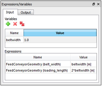 Figure 4: Expressions/Variables panel, Input tab showing one defined variable being used in two separate locations
Table 1: Expressions/Variables panel, Input tab options
Setting | Description | Range |
|---|---|---|
Variables | ||
Name | Enables you to specify a unique identifier for the variable. | The name must begin with a letter or underscore and can be followed by as many letters, underscores, or numbers as desired. Spaces and other symbols are not allowed. Letters are case sensitive. |
Value | The numeric value-or a function including other existing variable(s)-assigned to the variable name. | Any value; or any valid mathematical function including other existing variable(s), as long as the function does not create an infinite loop. (For more information about using functions, see Enter Input Variables or Mathematical Functions as Parameter Values.) |
Expressions | ||
Name | Lists the parameter field and location being used by the variable listed in the Value column. | Automatically provided. Cannot be edited. |
Value | Lists the variable Name and the units it is currently using within the field specified by the Expression Value column. | Automatically provided. Tip: Double-click the value to edit the units. (See also Change the Units for an Input Variable-or Functions Using Input Variables-in Use by a Field.) |
What would you like to do?
See Also:
Note: This method works only when using numerical values to define the variable. If for the variable definition, you want to reference other existing variable(s) within a function, you must define the new variable using the Expressions/Variables panel.
Ensure the units for the field are set the way you want. Important:Though the variable itself will be saved without units, its use in this particular field will be affected by the units that are displayed during the next step.
Directly into the field in which you want to use the variable, enter a name for the new variable, and then press Enter. Tips: The name must begin with a letter and must have no spaces. Only letters, numbers, and underscores are recognized (no symbols). Letters are case sensitive. The nme must not include pre-defined mathematical functions nor constants.
In the Variable Creation dialog, enter a numerical value for the variable, and then click Create variable. You will notice all of the following events:
The variable name is replaced by the numerical value in the parameter field. The variable is also using the units that were set for that field when the variable was entered. Tip: Double-click the field to see the full variable name and the units that it is using.
The new variable is displayed in the following two places on the Input tab of the Expressions/Variables panel (from the Tools menu, click Expressions/Variables):
Under Variables, where it is saved without units for use in other parameter fields. Tip: You can edit both the name and the value by double-clicking the information you want to change. (See also Edit the Name of an Existing Input Variable or Edit the Value of an Existing Input Variable.)
Under Expressions, where the variable name and units applied in that particular usage are saved along with the location of its use. Tip: You can edit the value and units recorded here by double-clicking the information in the Value column, and then modifying anything before the closing bracket.
See Also:
From the Input tab on the Expressions/Variables panel (from the Tools menu, click Expressions/Variables), double-click the Value for the variable Name you want to change. The Value field for that variable becomes active.
Enter the new value you want and then press Enter. The new value is saved. Notes:
The variable value is always saved without units. When used in a field, this variable will use in that instance whatever units are currently being displayed for that field.
Once used in a field, you cannot change from the field the units being used by the variable in that particular field. (See also Change the Units for an Input Variable—or Functions Using Input Variables-in Use by a Field.) You can, however, change the units by modifying the Value information in the Expressions/Variables panel under Expressions. Just double-click the Value you want to change, and then modify anything you want before the closing bracket.
See Also:
From the Input tab on the Expressions/Variables panel (from the Tools menu, click Expressions/Variables), double-click the Name for the variable you want to change. The Name field for that variable becomes active.
Enter the new name you want and then press Enter. The new name is saved in the panel and is also replaced in any field making use of the variable.
See Also:
Do one of the following:
In the Expressions/Variables panel under Expressions, find the instance of the variable whose units you want to change, double-click the Value for that usage, and then modify the units displayed in the brackets.
Remove the variable name-or function using the variable name-from the field, set the units for the field to the ones you want adopted by the variable or function, and then re-enter the variable name-or function using the variable name-again. Tip: Double-click the field to see the full variable name-or function using the variable name-and the units that it using in that instance.
See Also:
From the Input tab of the Expressions/Variables panel, select the Name of the variable you want to remove, and then click the Remove button. Just that variable is removed from the list.
Note: The last value replaces the variable name in any parameter field the removed variable was being used, and the Expressions list recording for that variable is cleared.
See Also:
From the Input tab of the Expressions/Variables panel, select a variable to enable the buttons, and then click the Remove All button. All the variables in the list on that tab are removed from the list.
Note: The last values replace all the respective variable names in any parameter field the removed variables were being used, and the Expressions list recordings for the all the variables are cleared.
See Also:
Defining output variables enable you to distill a set of data points from a Property or Curve into a single final value.
What would you like to do?
See Also:
Output variables enable you to distill a set of data points from a Property or Curve into a single final value. (See also Use Properties and Curves.) This process is illustrated in the example provided in Figure 1 below.
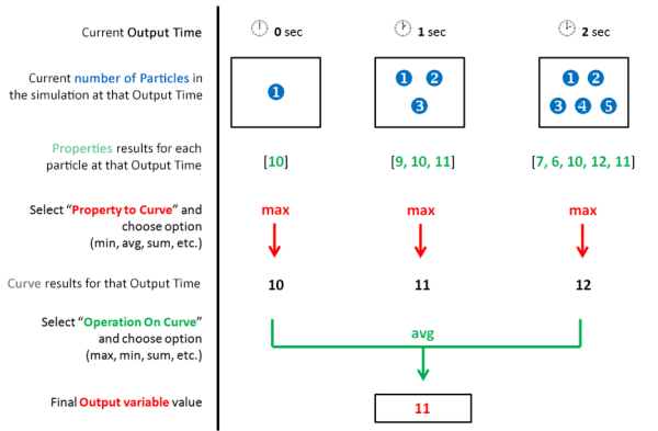 Figure 1 : Example of how Output variables are distilled into one value from a data set you define
In this example, the output time for the data set is limited to the first three seconds of the simulation, which then gives us the number of particles available at each of those three outputs. Then, the Property value for each particle at each of the three outputs is provided. Those Property values are then distilled into a single-value Curve for each output time, in this case the maximum value out of each of the three Property data sets is selected. Out of the three resulting Curve values, one last distillation, in this case by average value, gives us the final value that will be saved to the Output variable, in this case, 11.
You can use Output variables as an alternative to generating and measuring data in Time plots. (See also About Graphing (Plot or Histogram) a Data Set Within Rocky). Unlike a Time plot, an Output variable allows you to distill a set of Property or Curve values into a single value in one, easy-to-find location. For example, this method would be a benefit when needing to calculate the average mass of particles in a particular cube-shaped portion of the simulation between 3 and 10 seconds simulation time. (See also Filter Views and Data with User Processes.)
You can also use Output variables to distill data into a single value for exporting out of Rocky and into an Ansys Workbench project. When used together with Rocky's Input Variables, Workbench's Design Points functionality enables you to replace Input Variables from Rocky with new values, and then have Rocky provide the resulting Output value, all of which helps you more easily iterate upon simulation and setup components.
Tip: To see walk-through examples of using Output Variables within Workbench-connected projects, refer to the following Tutorials:
Use the images and table below to help you understand how to define Output variables.
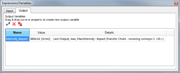 Figure 2: Expressions/Variables panel, Output tab showing one defined Property variable

Table 1 : Expressions/Variables panel, Output tab and Edit Properties dialog options
Setting | Description | Range |
|---|---|---|
Name | Enables you to specify a unique identifier for the variable. By default, it is the name of the Curve or Property that you have chosen but can be edited as desired. | The name must begin with a letter or underscore and can be followed by as many letters, underscores, or numbers as desired. Spaces and other symbols are not allowed. Letters are case sensitive. |
Value | The numerical value assigned to the variable as determined by the Curve or Property that you have chosen and the constraints you have assigned. | Automatically calculated based upon the settings you have chosen. |
Details | A summary of the constraints imposed upon the Curve or Property that results in the Value displayed. | Automatically listed based upon the settings you have chosen. |
Property to Curve | When the variable is based upon a Property, this is the function that will convert the Property values at each output time in the Domain Range to a single value. This single value will then be acted upon by the Operation on Curve function to get the final Value. | Min; Max; Average; Sum; Sum Squared; Variance; Standard Deviation For more information, see Use Properties and Curves. |
Operation on Curve | If the variable is based upon a Curve, this is the operation that will be applied to it to generate the final Value for the variable. If the variable is based upon a Property, this is the operation that will be applied to the single value generated from the Property to Curve value to achieve a final Value for the variable. | Min; Max; Average; Sum; Sum Squared; Variance; Standard Deviation For more information, see Use Properties and Curves. |
Domain Range | Defines what Output Times of the simulation are included in the final Value calculation. The options are as follows:
| Application Time Filter; All; Last Output; Time Range; Specify Time; After Time; Time Range Relative to Simulation End |
Initial | When Time Range or After Time is chosen for Domain Range, this is the starting time to begin calculations. | Any value between 0 and the final simulation time. |
Final | When Time Range is chosen for Domain Range, this is the ending time when calculations are stopped. | Any value between the Initial time and the final simulation time. |
At Time | When Specific Time is chosen for Domain Range, this is the exact moment in which the calculation will be performed. | Any value between 0 and the final simulation time. |
Range from end | When Time Range Relative to Simulation End is chosen for Domain Range, this is the period of time before the final simulation time in which output times will be included in the calculation. For example, when you want to include only the last X seconds of the simulation. | Any value between 0 and the final simulation time. |
What would you like to do?
See Also:
Set up and process the simulation as you normally would.
Do all of the following: - Select the Curve or Property tab that contains the information you are interested in. (From the Data panel, select Particles, the geometry, or user process for which you want data and then in the Data Editors panel, select the tab for which you are interested.) - Click and drag the Name of the data you want to the Output tab of the Expressions/Variables panel. (From the Tools menu, click Expressions/Variables.) - Release the mouse. The data appears as a new variable in the Output list.
See Also:
From the Output tab of the Expressions/Variables panel, select the Name of the variable you want to edit, and then click the Edit button.
From the Edit Properties dialog, enter the information you want as explained in Table 1, and then click OK.
See Also:
From the Output tab of the Expressions/Variables panel, select the Name of the variable you want to remove, and then click the Remove button. Just that variable is removed from the list.
See Also:
From the Output tab of the Expressions/Variables panel, select a variable to enable the buttons, and then click the Remove All button. All the variables in the list on that tab are removed from the list.
See Also:
Recording or writing PrePost Scripts and then playing or using them in Rocky are great ways to save time by automating repeatable tasks.
What do you want to do?
See Also:
Creating and using PrePost Scripts in Rocky is a great way to save time by automating repeatable tasks. Scripts can be recorded and played in the PrePost Script panel, added to the PrePost Scripts list under the Solver entity, and can be launched from the command line (see also Use the Command Line to Play a Script).
How you choose to create a script depends upon the task you are trying to repeat, and your level of familiarity with both Python and Rocky's API:PrePost functionality (see also Customize and Extend Rocky with Python). Specifically:
If the set of steps you want to repeat can be limited to things you click or enter in the Rocky UI, recording a script in the PrePost Script panel might be your easiest and quickest choice.
If you require more control over inputs or want access to tasks not directly accessible from the Rocky UI, then writing a script in Python may work better for your needs.
See the sections below for more detail.
When you choose to start recording a script from the PrePost Script panel, every step you take in Rocky is remembered until you choose to stop the recording. Then, you can choose to "play" your script within other parts of the set up, another view, or even other simulation files to repeat the same recorded steps automatically.
For example, you can use recorded scripts to accomplish all of the following tasks:
Create the very same Animation Key Frame sets in other simulations
Create a common variable set for use in other simulations
Apply custom graph views to your plot window that use your preferred units and grid settings
Export a set of animation key frames to individual image files
Apply your preferred visualization settings to other 3D View windows within your same simulation
When you record a script using the PrePost Script panel, Rocky automatically saves the resulting PY file in the correct folder location and using the required script_ prefix.
Tip: As long as your script PY file begins with script_ and is saved in either the ..RockyScripts folder (for scripts shared across projects) or the ..<ProjectName>rocky.filestmpmacros-0 folder (for current-project-only scripts) (see also File Types and Folders in Rocky), it can be listed and played in the PrePost Script panel.
You can also write and edit scripts outside of the Rocky program, and then apply them to your simulations in Rocky-either by playing the resulting PY file from the PrePost Script panel, or by pasting the code directly into the Python Shell panel.
To write or edit a script, knowledge of both Python (see also Customize and Extend Rocky with Python) and Rocky's API:PrePost functionality (see also I cannot find Rocky API documentation) is required.
Tips:
Gain hands-on experience with creating and using scripts by following either Tutorial - Static Angle of Repose Test in the Rocky Tutorial Guide or Tutorial - Tablet Coater in the Rocky Tutorial Guide.
View and modify sample scripts in the PrePost Scripts Repository section on the Rocky Customer Portal. (If you do not already have sign-in information for the customer portal, please contact your Rocky representative for assistance.)
Rocky enables you to share your recorded and saved scripts across different Rocky projects, or use them for only the current project. Scripts saved to the Scripts shared across projects tab will be available for all your Rocky projects across the application; scripts saved to the Project scripts tab will appear only in the current project (Figure 1).
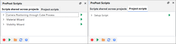
The tab you have selected when you choose to record your script (see also Record a New Script) or import your script (see also Add an External Script File to the Scripts Directory) determines the category to which the new script will be assigned. Scripts can be copied from one tab to another through the right-click menu (see also Copy a Script).
Note: Only scripts on the Project scripts tab are saved during archiving (see also Archive a Simulation Project) and are shown on the PrePost Scripts entity under Solver (see below.)
Any scripts that you have saved to the Project scripts tab are eligible for running automatically before and/or after simulation processing through the PrePost Scripts sub-entity on the Data panel under Solver (Figure 2). In this way, you can further automate your setup and post-processing, especially in situations where you are running many similar kinds of cases.

In this version of Rocky, only scripts that are compatible with the Python 3 (PY3) language will be supported. This means that some scripts that worked in older versions of Rocky may need to be recreated or modified to support the Python 3 guidelines. (See also My old script no longer works.)
In addition, only PY files starting with script_ will be eligible to play in the PrePost Script panel. Script files without this prefix can still be applied by copying and pasting the code into the Python Shell panel.
Use the images and table below to understand how to create and apply scripts.

Table 1: PrePost Script panel button descriptions
Button | Description |
|---|---|
| Starts the recording process, which is the first step to creating a new script. Saves each step in Rocky until you press the Stop and Save Script button. Note: The tab you have selected when you click Record Script determines what kind of script is created-a script shared across all projects, or a script saved only for this project. |
| Stops the recording process and saves the steps that were taken. |
| Applies the recorded steps of the selected script to whatever element is currently active in the Rocky UI. |
| Opens the tab-specific (shared across project or just current project) Scripts folder where the script PY files are saved. From here, you can choose to do any of the following:
Note: The tab you have selected when you click Open PrePost Scripts Directory determines which scripts folder is opened-the folder containing scripts that are shared across all projects, or the folder containing scripts saved only for this project. |
| When scripts are added to or removed from the directory, this refreshes the list in the PrePost Script panel to include any newly added or removed PY files. |
| Opens a short Help file with instructions for how to use the PrePost Script panel. |


What do you want to do?
See Also:
Ensure the PrePost Script panel is displayed. (From the Tools menu, click PrePost Script.)
From the PrePost Script panel, do one of the following: - To record a script that can be shared across all other Rocky projects, ensure the Scripts shared across projects tab is selected. - To record a script that can be used only for this project, ensure the Project scripts tab is selected.
Tip: If you change your mind, you can copy the script to the other tab later. (See also Copy a Script.)
Click the Record Script button.
From the New PrePost Script dialog, enter a name for the script you want to create, and then click OK. The new script name appears on the selected PrePost Script panel tab and the button changes to the Stop and Save PrePost Script button.
In the Rocky UI, perform the steps of the task that you want to repeat.
When the steps are complete, from the PrePost Script panel, click the Stop and Save PrePost Script button.
See Also:
Use this procedure to add a script to the Scripts directory.
Copy the PY script file that you want to add. Tip: In order for Rocky to recognize it and have it show within the PrePost Script panel, the script file name must begin with script. For example: script_video settings.py Note: A Rocky script not named in this exact way may still be used but will not be listed within the PrePost Script panel. Instead, these scripts must be launched from outside of Rocky. (See also Use the Command Line to Play a Script.)
Ensure the PrePost Script panel is displayed. (From the Tools menu, click PrePost Script.)
From the PrePost Script panel, do one of the following: - To add the script in a way that it can be shared across all other Rocky projects, ensure the Scripts shared across projects tab is selected. - To add the script in a way that can be used only for this project, ensure the Project scripts tab is selected.
Click the Open PrePost Scripts Directory button.
Into the file directory location that opens, paste the PY file you copied in step 1.
See Also:
Ensure that the script you want to apply has been saved to the correct directory. (See also Add an External Script File to the Scripts Directory.)
Within the Rocky UI, select the component to which you want the recorded steps of the script applied.
From the PrePost Script panel, select the name of the script you want applied, and then click the Playback PrePost Script button. The recorded or scripted steps are taken on the selected component. Tip: To see an overview of the script's processes, click the expand arrow to the left of the script's name. Click the arrow again to contract it.
Note: You can also have scripts applied automatically either directly before and/or after the simulation is processed. (See also Automatically Apply Scripts Directly Before or After Processing.)
See Also:
Ensure that the scripts you want to automatically apply either directly before and/or after your simulation is processed are listed on the Project scripts tab of the PrePost Script panel. (See also Copy a Script.)
From the Data panel, expand the Solver entity, and then click PrePost Scripts.
From the Data Editors panel, do the following:
In the Run before simulation box, enable all the scripts you want to automatically run directly before the simulation is processed.
In the Run after simulation box, enable all the scripts you want to automatically run directly after the simulation is processed.
Tip: You can also manually apply scripts at any time during your Rocky project. (See also Manually Apply a Saved Script.)
See Also:
From the PrePost Script panel, select the tab containing the script you want to edit.
Click the Open PrePost Scripts Directory button.
From the directory dialog, right-click the script file you want to edit, open it with your favorite Python editor, modify it as desired, and then save the file as a PY extension. Notes:
In order for Rocky to recognize it and have it show within the PrePost Script panel, the script file name must begin with
script_. For example:script_video settings.pyA Rocky script not named in this exact way may still be used but will not be listed within the PrePost Script panel. Instead, these scripts must be launched from outside of Rocky. (See also Use the Command Line to Play a Script.)To work properly in this version of Rocky, the Python 3 programming language must be used. (See also My old script no longer works.)
Tip: Scripts also have access to the Rocky's API:PrePost functionality, which can be explored in the following ways:
By using the Python Shell panel. (From the Tools menu, click Python Shell.) (See also Customize and Extend Rocky with Python.)
By using the Contents, Search, or Index tabs within the API:PrePost Manual. (From the Rocky Help menu, point to Manuals and then click API:PrePost Manual.)
See Also:
Ensure the PrePost Script panel is displayed. (From the Tools menu, click PrePost Script.)
Ensure also that you have saved your Rocky project. (See also Save a Simulation Project.)
From the PrePost Script panel, do one of the following:
To copy a shared script to the current project folder, select the Scripts shared across projects tab. Tip: Follow this procedure if you want to do either or both of the following:
Automatically apply a script either directly before and/or after the project is processed. (See also Automatically Apply Scripts Directly Before or After Processing.)
Include the script in your Rocky Archive. (See also Archive a Simulation Project.)
To copy a current project script to the folder shared with all other projects, select the Project scripts tab.
Right-click the name of the script you want to copy, and then click Copy Prepost Script to project. The script you selected now appears on the other PrePost Script panel tab. In addition, any copies on the Project scripts tab now also appear on the Solver PrePost Scripts list. (See also Automatically Apply Scripts Directly Before or After Processing.)
See Also:
From the PrePost Script panel, select the tab containing the script you want to remove.
Right-click the name of the script you want to remove, and then click Remove. The script name is removed from the PrePost Script panel. The script PY file is also removed from the Script directory. If the script was removed from the Project scripts tab, then it was also removed from the Solver | PrePost Scripts boxes. (See also Automatically Apply Scripts Directly Before or After Processing.)
See Also:
Note: Renaming a script affects only what is shown in the Rocky UI. It does not change the PY file name that is saved in the PrePost Scripts directory.
From the PrePost Script panel, select the tab containing the script you want to rename.
Right-click the name of the script you want to rename, and then click Rename.
From the Renaming PrePost Script dialog, enter a new name for the script, and then click OK. The script's new name appears in the PrePost Script panel. If the renamed script was on the Project scripts tab, the name in the Solver | PrePost Scripts boxes are also updated accordingly. (See also Automatically Apply Scripts Directly Before or After Processing.)
See Also:
Once you save a copy of your partially processed simulation (see also Save a Copy of a Partially Processed Simulation for Restart Purposes), you are able to change or delete existing boundaries and/or Particle sets as well as add new ones.
However, to preserve the integrity of the original simulation, Rocky limits the setup parameters that you can change for existing geometries and Particle sets to only a select few.
What would you like to do?
See Also:
After saving a copy of a partially processed simulation for restart purposes (see also Save a Copy of a Partially Processed Simulation for Restart Purposes), you can add additional geometries and Particle sets but will be unable to change some settings for existing geometries, inlets, and particles due to the way they affect the calculations that are already in process. Most other settings will be unaffected in the copy and can be modified as usual (Table 1).
Note: If you have saved for restart purposes a copy of a partially processed simulation that had both breakage enabled and broken fragments within the simulation at the time you saved your copy, the fragments will not be present in the copy you want to restart due to a limitation between the features. However if you choose to restart processing the simulation copy, breakage should work in the newly processed output times. (See also Enable Particle Breakage Calculations.)
See the sections below for further detail on what settings and parameters are editable within a copy of a partially processed simulation.
Since any Volume Fill Input will inject all of its particles immediately after the simulation begins, and a simulation must have particles in it to be saved for restart, the particles injected from a Volume Fill input will still appear in the copy. However, because the injection has already completed, the settings for any existing Volume Fill inputs will be disabled. You are able to add new Volume Fill inputs or duplicate any existing Volume Fill inputs as needed.
Any Continuous Injection or Custom Inputs (see also About Adding and Editing Particle Inputs) you had in the original simulation that were active at the time the copy was saved will still appear in the copy. And while these copied inputs and the Particle sets assigned to them cannot be removed from the copy, there are ways you can disable them if you no longer want to use them in the simulation moving forward.
Tips:
If you do not want an individual Particle set within a copied Continuous Injection input to be released in the simulation copy, you can set the Mass Flow Rate of that Particle set to zero.
If you have set all of the Particle sets within an individual Continuous Injection input to have zero as their Mass Flow Rates, you may choose to include a second Particle Input using the same Entry Point as the first, as long as all of the Mass Flow Rates in the first Input are zero, and all the Mass Flow Rates in the second Input are greater than zero.
Any Motion Frames (see also About Creating and Applying Motion Frames) you had in the original simulation that were active at the time the copy was saved will still appear in the copy and will retain their original geometry assignments. However, even though the geometries using the frames can be removed, the copied frames themselves cannot be removed from the copy, and will also only allow changes to the Stop Time field for the existing motion (as long as the copied motion hasn't completed yet, meaning the Stop Time value is positive); new motions can be added to the existing frame, however, by clicking the Add Motion button. In addition, only new motion frames can be assigned to new geometries in the copy; newly added geometries cannot be assigned frames copied from the original simulation, and geometries with motion frames copied from the original simulation cannot be assigned newly added motion frames.
Tips:
If you do not want a copied motion to occur in the copy, or want to define a new kind of motion for the copied geometry that is assigned the copied frame, you can set the Stop Time of the copied motion in the copied frame to zero (0), and then create a new motion (click the Add motion button) within the existing frame if desired. Note: Setting the Motion Frame Stop Time to zero (0) disables the field from being changed further. If you need to edit the Stop Time, press the Undo button (see also Undo or Redo a Single Action at Once) to re-enable the field.
If you want to change the motion assignment of an existing geometry, import a new copy of the geometry, create a new motion frame, and then assign the new motion frame to the new geometry. You can then delete the old geometry if you choose.
If you want to assign a copied motion to a newly added geometry, make a copy of the old motion frame and then assign that to the new geometry.
The following table attempts to document what Rocky settings are able to be changed in a copy of a partially processed simulation.
Table 1: Editable Settings When Restarting a Simulation
DATA PANEL SECTION | EDITABLE SETTINGS | CONDITIONS/NOTES | SEE ALSO |
|---|---|---|---|
STUDY | |||
Study | All settings are editable. | None. | |
PHYSICS | |||
Physics | All settings are editable. | None. | |
GEOMETRIES | |||
Feed Conveyor; Imported Geometry | Just the Thermal Boundary Type. | For existing feed conveyors and imported geometries. | About Feed Conveyor Parameters ; |
Feed Conveyor | Just the Belt Profile settings (excluding the number of rolls) and the Belt Motion settings. | For existing feed conveyors that have released particles. | About Feed Conveyor Parameters |
Feed Conveyor; Inlet | All settings are editable. | For feed conveyors or inlets that have not yet released particles. | About Feed Conveyor Parameters; About Inlet Parameters |
Receiving Conveyor | All settings are editable. | None. | About Receiving Conveyor Parameters |
Imported Geometries |
| Only these settings can be edited on already imported geometries. However, for newly imported geometries all settings are editable. | |
MOTION FRAMES | |||
Motion Frames | Just the Stop Time. | For any existing motion of an existing Motion Frame that is in process or has yet to happen. | |
MATERIALS | |||
Materials | All settings are editable. | None. | |
MATERIALS INTERACTIONS | |||
Materials Interactions | All settings are editable. | Editing these settings will affect the previously released particles what may lead to unrealistic behavior. Please, evaluate the results carefully. | |
SPH | |||
SPH |
| None. | |
SPH > Eulerian Solution | Enable Eulerian Solution. | None. | |
Fluid Inlet | Just the Stop Time. | None. | |
Outlet | All settings are editable. | None. | |
PARTICLES | |||
Particles | Just the Rolling Resistance; and the Enable Rotations. | Only these settings can be edited on existing particles. However, for newly particles all settings are editable. | |
PARTICLE INPUTS | |||
Continuous Injection | Just the Stop Time. | For existing inlets and feed conveyors that have released particles, as long as the Stop Time value is greater than the original simulation time represented by the current output time. | |
CFD COUPLING | |||
CFD Coupling | All settings are editable. | None. | |
DOMAIN SETTINGS | |||
Domain Settings | All settings are editable. | None. | |
SOLVER | |||
Solver | All settings are editable. | None. | |
PARTICLES CALCULATIONS | |||
Particles Calculations | All settings are editable. | None. | |
USER PROCESSES | |||
User Processes | All settings are editable. | None. | |
COLOR SCALES | |||
Color Scales | All settings are editable. | None. |
Note: If you need to modify any of the above settings, saving a copy of the processed simulation might not work for you. Instead, return to your original simulation and reset it before changing any of the above parameters.
What would you like to do?
See Also:
Process and save part of a processed simulation. (See also Save a Copy of a Partially Processed Simulation for Restart Purposes.) The copy will open with the Time toolbar slider reset to zero (0). However, the simulation will be processed to the last output time that you selected in the original simulation.
Using the lists of what you can and cannot change for guidance (see also About Changing Geometries and/or Particles in a Partially Processed Simulation), change and/or delete existing boundaries, add new boundaries, and/or add new Particle sets as you want.
Process and analyze the simulation as you normally would.
See Also:
Use this section to quickly find and perform common tasks in Rocky.
What would you like to do?
Enter Input Variables or Mathematical Functions as Parameter Values
Change Set Up Parameters in a Partially Processed Simulation
Use the 1-Way Fluent Method to Process Fluent and Rocky Simulations
Use the 2-Way Fluent Method to Process Fluent and Rocky Simulations
Reuse 3D View Window, Workspace, and User Process Setups in Other Projects
See Also:
You can create Input variables in Rocky (see Defining Your Variables) and then use them in place of actual numerical values in situations where you want more flexibility. These variables can be used alone or within functions.
Tip: Rocky includes several visual feedback mechanisms, like text color, to help you ensure the variable names and mathematical functions you enter are correct. See Use Colored Text to Validate the Syntax of Your Entries for more information.
Important:Verify that your field units are set the way you want before using a variable-or function using a variable-within a field. Even though variables are always saved in the Variables list without units, as soon a variable-or function using a variable-is used within a parameter field, it takes on whatever units are currently set for that field and then those units are recorded for that specific usage in the Expressions list. Changing the units for the field after the variable or function have already been entered only converts the numerical display to reflect the new units; the original variable or function amount and units are still retained. However, you can change the units and value later by editing it in the Expressions list.
Most text fields in Rocky support entering variables or mathematical functions as parameter variables, including three-part text fields. There are a few exceptions to be aware of, however. (See also I cannot enter an input variable or mathematical function into a text field.)
Most of these parametric expressions will be retained while saving a copy of a project for restart purposes, but there are a few exceptions for some Start Time and Stop Time fields. (See also I get a "Links removed" message when I save my project for restart purposes.)
Most text fields will also support the entering of pre-defined mathematical functions (e.g., floor and pow) and constants (e.g., pi and e) that come standard with Python-based programs, including Rocky. And as such, these particular functions and constants cannot be used when defining Input variables.
What would you like to do?
See Also:
Using the Data and Data Editors panels, locate and select the field for the parameter you want to replace, exactly enter the name of the variable you want to use, and then press Enter. The current value set for the variable in the Expressions/Variables panel is displayed in the field.
Tip: To see the units that are set for the variable you used, double click the value in the field. The units are displayed in brackets [ ] after the variable name.
Note: You cannot use pre-defined functions or constants to define your variable.
See Also:
Using the Data and Data Editors panels, locate and select the field for the parameter you want to replace, and then enter the function you want to use.
See Also:
Using the Data and Data Editors panels, locate and select the field for the parameter you want to replace, and then enter the pre-defined mathematical function or constant you want to use.
See Also:
You can change the speed of a default receiving or feed conveyor at any point during the simulation. For example, you might want to measure reclaiming belt power by starting off a simulation with a feed conveyor stopped until a hopper is filled with particles, and then ending the simulation with the conveyor up to full speed.
Ensure the default conveyor for which you want to change belt speed has already been added. (See also Add and Edit Geometry Components.)
From the Data panel, under Geometries, select the Receiving Conveyor or Feed Conveyor for which you want to change belt speed. The parameters for that geometry are displayed in the Data Editors panel.
From the Data Editors panel, on the Receiving Conveyor or Feed Conveyor tab, ensure the Belt Motion sub-tab is selected, and then do all of the following:
In the Belt Speed box, enter the full speed you want the belt to reach after acceleration is complete.
In the Beginning Start Time box, enter the amount of time that you want the simulation to run before the belt starts accelerating.
In the Acceleration Period box, enter the amount of time you want the belt to increase from full stop to full Belt Speed.
In the Beginning Stop Time box, enter the amount of time that you want the simulation to run before the belt starts decelerating.
In the Deceleration Period box, enter the amount of time that you want the belt to decrease from full Belt Speed to full stop.
See Also:
You change particle adhesion when you want a particle to act wetter or "stickier" than normal during a simulation. This might be useful in showing how ore flows through handling equipment during the wet season as compared to the dry, for example.
Tip: It is good practice to calibrate your particle settings to the real-world behavior of the material you are simulating before changing settings like adhesion. You may wish to use the Material Wizard and/or the Calibration Suite to help you with this task.
Set up the simulation as you normally would. (See also Setting Up a Simulation.)
During the Set Simulation-Wide Parameters step, ensure you select both the Rolling Resistance Model and the Adhesive Force you want from the Physics | Momentum tab. (See also About Physics Parameters.)
Adjust Materials Interactions values by doing all of following:
From the Data panel, select Materials Interactions.
From the Data Editors panel, choose the materials you want to modify from the Select Materials lists.
Adjust one or all of the settings provided including friction, adhesive distance, and force and/or stiffness fractions. (See also About Modifying Materials Interactions and Adhesion Values.)
Adjust Rolling Resistance values by doing all of the following:
From the Data panel, under Particles, select the rigid, convex Particle set for which you want to change adhesion.
From the Data Editors panel, select the Movement tab, and then adjust the Rolling Resistance value. Notes: - The Type C: Linear Spring Rolling Limit Rolling Resistance model is recommended for sticky particles. (See also About Physics Parameters.) - Rolling Resistance is not usually needed for shaped particles.
Process the simulation and then continue to adjust the Materials Interactions and Rolling Resistance values until you get the results you want.
See Also:
You set a particle size range-otherwise known as a Particle Size Distribution (PSD)-when you want particles of one shape but different sizes to be used in the simulation. If you set more than one size for a Particle set, Rocky uses a calculation to specify the distribution of sizes within any two dimensions you specify. This helps to more accurately reflect real matter.
When setting size ranges, the following three methods, or Size Types, can be used as a basis for defining your particle sizes (Figure 1):
Sieve Size (formerly "Sieve"), which for especially default Rocky shapes, bases particle size upon a virtual mesh hole just big enough for the particle to pass through. Note: Due to the way Sieve Size is calculated, it should be used only for even and balanced particle shapes (such as the default Solid particles included with Rocky) and not for fibers or shapes with high aspect ratios. (For more detail on how Sieve Size is calculated in Rocky, see the DEM Technical Manual. (From the Rocky Help menu, point to Manuals, and then click DEM Technical Manual.))
Equivalent Sphere Diameter (formerly "Equivalent Diameter"), which for especially irregular objects, bases particle size upon the diameter of a sphere with equivalent volume.
Tip: To see a walk-through example of setting and using Equivalent Sphere Diameter, refer to the following Tutorial: Tutorial - Windshifter in the Rocky Tutorial Guide. Original Size Scale, which for especially imported shapes, bases particle size upon the original size of the shape.
Tip: To see a walk-through example of setting and using Original Size Scale, refer to the following Tutorial: Tutorial - Tablet Coater in the Rocky Tutorial Guide.

The PSD in Rocky is linear by Particle Mass or, on a semi-log scale, by Particle size and not by number. When you enter the percentage of cumulative mass and then either particle sieve Size, sphere Diameter, or original size Scale Factor (representing the three available Size Types, respectively), these represent points on a semi-log plot. Anything between two points follows the linear rule:

(See also About Adding and Editing Particle Sets.)
For example, if you specify 0.1 and 0.05 (m) particle sizes measured by sieve size, you will get a range of various particle sizes within those two dimensions.
Use the image and procedure below to set size ranges for your Particle sets.

Ensure that the Particle set for which you want to specify size ranges has been added. (See also Add a New Particle Set.)
From the Data panel, select the Particle set you want (for example, Particle <01>) and then from the Data Editors panel, select the Size tab.
Set what you want for Size Type. (See also About Adding and Editing Particle Sets.)
Click the Add button once for each additional size range you require. Note: For rigid particles composed of Single Elements, there is no limit to the amount of rows you can add. For flexible or rigid particles composed of Multiple Elements (also known as *meshed* particles-see the Composition Tab section in the About Adding and Editing Particle Sets topic), only one row can be defined per Particle set.
Under Size, Diameter, or Scale Factor respectively, and starting with the first row, enter the maximum and minimum size values for each range in decreasing order. For example, to get a range of sieve sizes between 0.05-0.1 m and 0.01-0.05 m, enter 0.1, 0.05, and 0.01 in the first, second, and third rows respectively. (See Figure 2 above for example.) Note: The smallest value you enter (last row) will also be shown at that exact size (no range).
Under Cumulative %, starting with the second row, indicate what percentage of the total particle mass you want of that size value range by entering in decreasing order the previous row's percentage minus the percentage you want. For example, if you want 20% of the 0.05-0.1 m range, enter 80 (100-20); to get 60% of the 0.01-0.05 m range, enter 20 (80-20). (See Figure 2 above for example.)
Note: The percentage indicated in the final row also indicates what particle mass amount will be of that exact size (no range). For example, if the smallest size you enter is 0.01 m and you have entered 20 for Cumulative %, 20% of the particle mass will be exactly 0.01 m in size in addition to the ranges you have set.
See Also:
There are two primary ways you can use Rocky to gain an understanding of how your geometries will wear over time. One way is by enabling surface wear modification, which changes the physical appearance of the geometry as the simulation progresses (Figure 1).
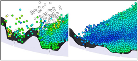
A second way is to turn on Boundary Collision Statistics (see also About Collision Statistics for Boundaries and then view a color map of the surface intensity (Figure 2), impact velocity, stresses, and more.
These features are independent of each other and are enabled from different areas of the Rocky UI. However, to view either type of wear data, you need to ensure that you have enabled enough geometry triangles prior to processing your simulation. Too few triangles will result in a jagged or blocky representation rather than a smooth one, but too many triangles can slow down your simulation.
Tip: To see a walk-through example of surface wear modification being using to analyze a SAG mill, review Tutorial - SAG Mill in the Rocky Tutorial Guide.
What would you like to do?
See Also:
One way you can use Rocky to gain an understanding of how your geometries will wear over time is by enabling surface wear modification. Turning this feature on for an imported geometry prior to processing changes the physical appearance of the geometry as the simulation progresses (Figure 1).
To view this type of wear data, you must ensure that you have enabled enough geometry triangles prior to processing your simulation. Too few triangles will result in a jagged or blocky representation rather than a smooth one, but too many triangles can slow down your simulation.
It is important to realize that this data is only collected after the Wear Start value on the Solver | Time tab is reached. This is to allow enough time for the particle flow within your simulation to reach a steady state before surface wear modification calculations begin.
Tips: To see walk-through examples of surface wear modification, refer to the following Tutorials:
Set up the simulation as you normally would. (See also Set Simulation Parameters). Tip: For easier comparison after the simulation is complete, consider including a copy of the imported geometry that will remain unworn. (See also Duplicate a Data Panel Item.)
Before processing the simulation, do all of the following:
From the Data panel, under Geometries, select the imported geometry for which you want to enable surface wear. The parameters for the geometry become active in the Data Editors panel.
From the Data Editors panel, on the Geometry tab, do all of the following:
From the Geometry sub-tab, ensure Triangle Size is small enough to enable the wear detail you want. (0.1 m is recommended for most chutes and mills).
From the Wear sub-tab, select the Wear Model you want to use, and then enter the Volume/Shear Work Ratio. Note: This is a calibration step that comes from real-world wear data you have collected on similar types of equipment.
From the Solver | Time tab, ensure that your Wear Start time is set to when you want wear data to be collected. (From the Data panel, select Solver and then from the Data Editors panel, locate this value on the Time sub-tab.) (See also About Solver Parameters.) Tip: It is best practice to set your Wear Start time to begin after a steady state has been reached for your particle flow.
Process the simulation as you normally would. (See also Processing a Simulation.)
From a 3D View window (see also About 3D View Windows), observe the changes to the surfaces of the geometry as the simulation progresses. Tip: If you included a copy of the original geometry in the simulation, you can use the unworn geometry as a comparison to one worn by surface wear modification.
Tips:
If you want to analyze the modified geometry outside of Rocky, you can choose to export it to an STL file. (See also Export a Geometry Component to an STL File.)
It is possible to save a copy of an in-process simulation with surface wear and have the wear calculations continue in the copy. (See also Save a Copy of a Partially Processed Simulation for Restart Purposes.) While you are unable to turn off wear calculations from the copy, if you no longer need wear, you can get around this by setting Volume/Shear Work Ratio to zero.
It is also possible to have wear calculations be made on replicated geometries.
See Also:
When you choose to turn on Boundary Collision Statistics (see also About Collision Statistics for Boundaries and enable wear-related categories such as Intensities, you are able to create and view a color map of the surface intensity (Figure 1), impact velocity, stresses, and more. These color maps can help you analyze the causes of excess wear on your conveyor belts or imported geometries.
Set up the simulation as you normally would. (See also Set Simulation Parameters.)
Before processing your simulation, ensure all of the following:
You have enabled the Boundary Collision Statistics that you want to be collected. (See also Enable and View Collision Statistics for Boundaries.)
You have verified that the default conveyor or imported geometry has its Triangle Size set small enough to enable the wear detail you want. (0.1 m is recommended for most chutes and mills). (From the Data panel under Geometry, select the component you want to verify. From the Data Editors panel, on the Geometry sub-tab, verify the Triangle Size value.)
Process the simulation as you normally would. (See also Processing a Simulation.)
Ensure you have a 3D View displayed in the Workspace. (See also Create and Modify a 3D View.)
When processing is complete enough to show the wear you want to visualize, from the first drop down list on the Coloring Settings toolbar, choose the data you want to display (e.g., Intensity.) The geometries in your simulation change color and a color legend is displayed in the 3D View.
Do any or all the following to adjust the view and color map details:
To better focus on the area you want to view, use the mouse to pan, rotate, and zoom. (See also About Using the Mouse and Keyboard to Change the View.)
To hide all items but the belt or geometry you want to focus on, use the eye icons to the left of the geometries and particles in the Data panel. (See also Show/Hide Components by Using Eye icons and Checkboxes.)
To modify the color bar, right-click the color legend and change the options listed. (See also About Color Scales.)
To focus on a different time period within the simulation, use the arrows or slider on the Time toolbar. (See also About the Time Toolbar.)
See Also:
There are five main steps to using the 1-Way Fluent CFD Coupling method to process a 1-Way coupled Rocky and Ansys Fluent simulation, as described below.
Tips:
You may also complete this process from within Ansys Workbench. To accomplish this with transient Fluent data, however, there are separate steps you must follow. (See also Set Up and Run a 1-Way Fluent Transient Project within Ansys Workbench.)
You may also complete this process without using the Fluent UI. (See also Use a Journal to Run Fluent and Export Transient 1-Way Results.)
Before beginning Step II below, ensure all of the following program requirements have been met:
A Rocky-supported version of Ansys Fluent is installed upon a machine that also contains a Rocky program installation. (See also System Requirements.) Note: Rocky does not need Fluent to be installed on the same machine in order to run a 1-Way Fluent simulation. However, Fluent needs Rocky to be installed on the same machine in order for Rocky to enable the Rocky Export menu item in Fluent.
If you are not certain whether you have installed the Ansys Fluent Coupling Support component during Rocky installation, first follow the Install Ansys Coupling Components procedure before beginning Step II.
In Ansys Fluent, set up the CFD simulation that you want to couple with Rocky. Important: Ensure that you complete all of the following; these exact settings are required for 1-Way Fluent coupled simulations:
From the Fluent Launcher dialog, do the following:
Under Dimension ensure 3D is selected.
Under Options select Double Precision.
From the Solution Methods tab, under Pressure-Velocity Coupling Scheme, ensure SIMPLE is selected.
Optional Steps:
If you want to use any standard Fluent post processing options, set them up now before processing the simulation.
If you want both sides of your coupled simulation to share identical geometries, set up those geometries now in Fluent, but be sure you save your Fluent Case File. Later in Rocky, you can choose to import those geometries directly from the CAS, CAS.H5, or CAS.GZ file that you will save from Fluent in the next step.
If you want both sides of your coupled simulation to share the same geometry movements, set up the translation or rotation movements now using Fluent Moving Meshes. These movements will later be imported (with the F2R file) into Rocky (Step IV.2 below), which will automatically convert them into Rocky Motion Frames. Note: If you chose to define your moving meshes in Fluent using expressions, you will need to set up your Motion Frames in Rocky manually. (See also Step IV.2 below and About Creating and Applying Motion Frames to Imported Geometries.)
From the File menu, Write the case to a location of your choosing. Tip: Remember the location of this directory as you will need to access files saved to it in later steps.
(Optional) Configure the options for Rocky Export by doing any or all of the following:
Define the directory you want to export by doing the following:
From the Fluent Rocky Export menu, point to Configure one-way export and then click Select Directory to Export.
From the Select folder to write fluent to rocky files, select the folder to where you want your fluid data saved, and then click Select Folder. Note: If you do not define this, Fluent will automatically use the same folder as your case file.
Define the additional variables you want to export by doing the following: Note: These additional variables can include static pressure, species variables such as mole fraction, diffusivity, and user defined memories. Other variables such as Velocity, Pressure Gradient, Temperature, and Fluid properties are always exported no matter what you select here.
From the Fluent Rocky Export menu, point to Configure one-way export and then click Select Variables to Export. Note: To do this task, you must first have variables defined within Fluent.
From the Additional Variables Selector dialog that appears, select the variables that you want included in the exported files, and then click OK.
Define how frequently you want files to be saved during the export by doing the following:
From the Fluent Rocky Export menu, point to Configure one-way export and then click Set Output Frequency.
b. From the Fluent to Rocky (F2R) time-step multiplier dialog define what you want for the F2R Time Step Multiplier value, and then click OK. Note: Only whole numbers are valid multipliers.
Export the data you want by doing one of the following:
To export steady-state data, do the following:
Process the CFD simulation until the fluid flow reaches a steady state.
From the Fluent Rocky Export menu, point to Export one-way data and then click Export current data to Rocky. Tips:
If you do not see this menu in Fluent, then first follow the Install Ansys Coupling Components procedure before continuing.
To perform this step before the Fluent case is done processing, stop Fluent from processing the case further before using Rocky Export menu.
An F2R and other files needed for coupling is saved to the same folder as your Fluent case file (or the alternate folder you defined in step 3).
To export transient data, do the following:
Begin the export process by doing one of the following:
To start recording from the initial conditions (without any prior Fluent results), initialize the Fluent case.
To start recording some time after Fluent results have been collected, process the CFD simulation until the fluid flow reaches the point that you want to start recording data, and then stop Fluent from processing the case further.
From the Fluent Rocky Export menu, point to Record one-way transient data, and then click Start one-way transient export. Tip: If you do not see this menu in Fluent, then first follow the Install Ansys Coupling Components procedure before continuing.
Begin (or resume) processing in Fluent until the point you want to stop recording data. Stop Fluent from processing the case.
From the Fluent Rocky Export menu, point to Record one-way transient data, and then click Stop one-way transient export. An F2R and other files needed for coupling is saved to the same folder as your Fluent case file (or the alternate folder you defined in step 3).
Click OK to close the confirmation message dialog.
Save the Fluent case again.
In Rocky, set up your simulation project as you normally would. (See also Set Simulation Parameters.) Tips:
If you want to use the exact same geometries as in the Fluent simulation, you may choose to import the CAS, CAS.H5, or CAS.GZ file you generated in Step II, which will include all available geometries as separate components.
If you enabled Energy Equations in the Fluent case, then ensure you also enable Thermal Modeling settings in Rocky. (See also Enable Thermal Modeling Calculations.)
From the Data panel, click CFD Coupling and then from the Data Editors panel, choose Fluent (Fluid → Particle) from the Coupling Mode list.
From the Select Fluent 2 Rocky export file dialog, locate and select the F2R file you exported in Step II, and then click Open. A new 1-Way Fluent item appears beneath CFD Coupling in the Data panel. Important:For F2R files that include transient data, this step could take several minutes to complete. In addition, if you chose to set up Moving Meshes in Fluent, one new Frame will appear under Motion Frames in the Data panel for each Cell Zone with motions you have defined. Important:If you have defined your Moving Meshes in Fluent using expressions, Rocky will not be able to create the associated Motion Frames for you automatically. Rather, you must manually create your own Motion Frames in Rocky to match the Fluent motions as closely as possible. Tip: To save loading time, the Nodes for the imported fluid are turned off by default in the 3D View. To see them, from the Coloring tab, enable the Nodes checkbox. (See also About Using the Coloring Tab to Change a 3D View.)
Under CFD Coupling, select the new item and then from the Data Editors panel, on the 1-Way Fluent tab, do the following:
Set the Start Time you want.
From the Interactions tab, do the following:
From the Particle list, select (or multi-select) the Particle set name(s) for which you want to define interactions, and then select the various CFD laws you want for the selected set(s).
Select what you want for Turbulent Dispersion.
(See also About Using the 1-Way Fluent Method.)
In Rocky, process the simulation as you normally would. (See also Start Processing a Simulation from the Beginning.)
See Also:
There are five main steps to using the 2-Way Fluent method to process a coupled Rocky and Ansys Fluent simulation, as described below.
Note: Both Single phase and Multiphase approaches are covered in this procedure.
Before beginning Step II below, ensure all of the following program requirements have been met:
A Rocky-supported version of Ansys Fluent is installed upon the same machine that contains your Rocky program installation. (See also System Requirements.)
If you desire to run Fluent as a parallel process (rather than a serial one), then the machine upon which you intend to run the Rocky portion of your coupled simulation must also run at least the host part of the Fluent process. (For more information about how the processing architecture works in Fluent, refer to your Ansys Fluent documentation.)
If you are not certain whether you have installed the Ansys Fluent Coupling Support component during Rocky installation, first follow the Install Ansys Coupling Components procedure before beginning Step II.
In Ansys Fluent, set up the CFD simulation that you want to couple with Rocky. Important:Ensure that you complete all of the following; these exact settings are required for 2-Way Fluent coupled simulations:
From the Fluent Launcher dialog, do the following:
Under Dimension ensure 3D is selected.
Under Options select Double Precision.
From the General tab, under Time select Transient.
From the Tree panel, expand Models, and then do one of the following:
To set up a CFD project with a single fluid phase, ensure that Multiphase model is set to Off.
Otherwise, to set up a CFD project with two or more fluid phases, do all of the following:
Under Models, select Eulerian. Note: The Volume of Fluid model is not supported by Rocky in this version.
Under Eulerian Parameters, keep all options cleared. (All are unsupported with coupling, including the Multi-Fluid VOF Model.)
Under Volume Fraction Parameters, select Implicit for Formulation.
Under Number of Eulerian Phases, select the number of phases that includes an additional one for particles. (The number of Eulerian phases should be set to number of fluid phases + 1.).
Click OK.
Only for projects where the Multiphase model has been set to Eulerian (i.e., multiphase simulations), ensure that you set the additional particle phase to have a different material from the primary phase.
Only for projects involving multiple fluid species, for the mixture-template for your Material Mixture, ensure that you have enabled Species Transport. Important:The species you list last in the Selected Species list is very important as Fluent considers it to be the bulk species; this last species, therefore, will not result in a mass source term from Rocky.
From the Solution Methods tab, under Pressure-Velocity Coupling Scheme, do one of the following:
For projects where the Multiphase model has been set to Eulerian (i.e., multiphase simulations), you must ensure that the Phase Coupled SIMPLE method is selected.
For projects where the Multiphase model has been set to Off (i.e., single phase simulations), you may choose any pressure-velocity coupling scheme that works for your particular application.
From the Solution Methods tab, under Transient Formulation, ensure that First Order Implicit is selected.
From the Run Calculation tab, under Time Advancement, do the following:
Set Type to Fixed.
Ensure the Time Step Size value you set matches the minimum initial Output Frequency you want for your Rocky and Fluent files. Tip: You can change the outputs to be less frequent than this minimum in your Rocky setup later.
Tip: To help ensure that you perform these setup steps correctly, please refer to the CFD Coupling Technical Manual document (from the Help menu, point to Manuals, and then click CFD Coupling Technical Manual). For single-phase approaches, you may also follow the self-guided:
Tutorial 14 - DEM-CFD Two-Way Coupling with Ansys Fluent.
Optional Steps:
If you want to start your Rocky simulation with a given initial fluid flow, save the solution in Fluent as a standard DAT (DAT.H5 or DAT.GZ) file to be used by Rocky later (see Step IV below). Note: If your simulation is multiphase, ensure that the secondary phase (particulate phase) has a volume fraction of zero set before saving your DAT (DAT.H5 or DAT.GZ) file. Later, after the simulation is initialized, the initial particulate volume fraction will be calculated in Rocky according to the particles enabled at the beginning of the simulation.
If you want to use any standard Fluent post processing options, set them up now before processing the simulation.
If you want both sides of your coupled simulation to share identical geometries, set up those geometries now in Fluent, but be sure you save your Fluent Case File. Later in Rocky, you can choose to import those geometries directly from the CAS, CAS.H5, or CAS.GZ file that you will save from Fluent in the next step.
If you want both sides of your coupled simulation to share the same geometry movements, set up the translation or rotation movements now using Fluent Moving Meshes. These movements will later be imported (with the CAS, CAS.H5, or CAS.GZ file) into Rocky (Step IV.2 below), which will automatically convert them into Rocky Motion Frames. Note: If you chose to define your moving meshes in Fluent using expressions, you will need to set up your Motion Frames in Rocky manually. (See also Step IV.2 below and About Creating and Applying Motion Frames to Imported Geometries.)
Write the completed CFD setup to a CAS (CAS.H5 or CAS.GZ) file.
In Rocky, set up your simulation project as you normally would. (See also Set Simulation Parameters.) Tip: If you want to use the exact same geometries as in the Fluent simulation, you may choose to import the CAS, CAS.H5, or CAS.GZ file you generated in Step II, which will include all available geometries as separate components.
Recommended: Save your Rocky project to the same folder in which you saved the CAS (CAS.H5 or CAS.GZ) file in Step II. (See also Save a New Simulation Project.)
Whether or not you choose to take this step, Rocky will create its own copy of the CAS (CAS.H5 or CAS.GZ).
Optional: If you want to start your coupled simulation with particle data already in the system, do all of the following:
Process the simulation as you normally would, without CFD coupling. (See also Start Processing a Simulation from the Beginning.)
After processing is complete, from the File menu, click Save project as….
From the Save As dialog, choose the third option, "Save as a New Project for Restart", and then click OK.
In the Save in list, choose the same location in which you saved the CAS (CAS.H5 or CAS.GZ) file in Step II, verify the File Name, and then click Save.
From the Data panel, click CFD Coupling and then from the Data Editors panel, choose 2-Way Fluent from the Coupling Mode list.
From the Select Fluent CAS file dialog, locate and select the CAS (CAS.H5 or CAS.GZ) file you generated in Step II, and then click Open. Important:A mesh validation step will occur immediately after the CAS file import. This requires a valid Fluent license on the same machine upon which you are running the Rocky simulation. After successful import, a new 2-Way Fluent item appears beneath CFD Coupling in the Data panel. In addition, if you chose to set up Moving Meshes in Fluent, one new Frame will appear under Motion Frames in the Data panel for each Cell Zone with motions you have defined. Important:If you have defined your Moving Meshes in Fluent using expressions, Rocky will not be able to create the associated Motion Frames for you automatically. Rather, you must manually create your own Motion Frames in Rocky to match the Fluent motions as closely as possible.
If the CAS (CAS.H5 or CAS.GZ) file imported new Motion Frames, assign each newly imported Frame to the geometry component you want to share corresponding movements with Fluent. (See also Apply a Motion Frame to an Imported Geometry.)
From the Data panel under CFD Coupling, select the new 2-Way Fluent item and then from the Data Editors panel, do all of the following:
From the Interactions tab, define the CFD laws you want per *Particle set* by selecting (or multi-selecting) the set name(s) from the Particle list, and then defining the laws you want for the selected set(s). From this tab, you can also set the Turbulent Dispersion options for the entire coupled simulation. (See also About Using the 2-Way Fluent Method.)
From the Coupling tab, define the Mapping Method and Sub-Stepping options you want.
From the Zones and Interfaces tab, do the following:
Select one or more options from the Coupling Fluid Cell Zone list.
(Optional) If provided, select the options you want from the Mapping Cell Zone Interfaces list.
From the Fluent tab, do all of the following:
Important: If your Fluent case is multiphase, from the Rocky Phase list, ensure that the phase representing particle flow is chosen.
Choose what fluid flow data Rocky starts with by doing one of the following:
To start your Rocky simulation without providing initial fluid flow data, ensure the Use Data Initialization checkbox remains cleared. Doing so ensures that the initialization settings prescribed in Fluent will be used to generate the initial fluid flow.
To start your Rocky simulation with initial fluid flow data, select Use Data Initialization, click the Import File button, and then select and open the DAT (DAT.H5 or DAT.GZ) file you saved in Step II. Important:If you chose to use initial fluid flow data in your simulation and your simulation is multiphase, you must have ensured that the secondary phase (particulate phase) had a volume fraction of zero set before you saved your DAT (DAT.H5 or DAT.GZ) file. This is important because later, after the simulation is initialized, the initial particulate volume fraction will be calculated in Rocky according to the particles enabled at the beginning of the simulation.
From the Version list, select what Ansys version you want to use for fluid coupling. Tip: If you do not see the Ansys version you expected, see also Rocky does not list my Ansys version when I try to set up 2-Way Fluent Coupling.
Choose how the fluid portion of the simulation is processed by doing one of the following:
To have it processed on only one processor on your local machine, from the Execution mode list, select Serial.
To have it processed on multiple processors on your local machine, from the Execution mode list, select Local Parallel and then from the Solver Processes field, enter the number of processors you want to dedicate to the CFD solver.
To have it processed across several machines on your network, from the Execution mode list, select Distributed Parallel and then do one of the following:
Under Hosts, click the Add button for each server you want to add and then for each row, define the Host name and Amount information.
To import an external list of hosts and amounts that you created outside of Rocky, click the Import File button, and then from the Import dialog, locate and select the TXT file containing the information, and then click Open. The Host section is populated with the information from the TXT file. Tip: The format for the TXT file needs to include the Host name repeated on separate lines for each Amount you want devoted. To see an example, create a few sample rows as specified directly above, click Export File and then save and view the results as a TXT file.
Choose how many Fluent files to keep by doing one of the following:
To keep each Fluent DAT (DAT.H5 or DAT.GZ) file (and in some cases, as with moving meshes, CAS files as well) for every Rocky output file that is saved, enable the Keep all files checkbox. Important:Unless you require all files for post-processing in Fluent, keeping all files is not recommended for the 2-Way Fluent method. (See also About Using the 2-Way Fluent Method.)
To keep only the last (or last several) Fluent DAT (DAT.H5 or DAT.GZ) files (and in some cases, CAS files) saved, ensure the Keep all files checkbox is cleared, and then enter the number of last-saved files you want to keep in the Files to keep box. Tip: Keeping the last 2 (or more) files is recommended. Important:If you decide to save fewer than all of the files, be aware that you will not be able to post-process the unsaved files in Fluent. Also, be aware that the number DAT (and in some cases, CAS) files you save will be as far back in time as you can restart your simulation since fluid data will not be available for prior times. Tip: You can also choose which quantities and frequency you want to write to disk using Fluent's Autosave functionality.
From the Variables tab, review the Additional Inputs and Additional Outputs (if applicable) that Rocky and Fluent will exchange during the coupled simulation. Tip: If you have enabled species transport, this is where the per-species variables Fluent provides Rocky, and the mass source terms Rocky provides Fluent will be listed.
Tips:
To verify or change the CAS (CAS.H5 or CAS.GZ) file selected, click Open (at the bottom of the 2-Way Fluent | Fluent tab) and Rocky will open its own copy of the CAS (CAS.H5 or CAS.GZ) file in Fluent. From here, you can view or make changes to the Rocky copy of the file. Important:Because Rocky uses only its own copy of the imported CAS (CAS.H5 or CAS.GZ) file, it is critical that you only open the imported CAS (CAS.H5 or CAS.GZ) from Rocky's Open button, and that you save any changes to the default location Rocky indicates.
If you make changes to the Rocky copy of the CAS (CAS.H5 or CAS.GZ) file in Fluent, click Refresh to have Rocky include the updates. Important:The Refresh button works only if you first opened the CAS (CAS.H5 or CAS.GZ) file from the Rocky Open button located at the bottom of the 2-Way Fluent | Fluent tab.
If you made changes to your original Fluent version of the CAS (CAS.H5 or CAS.GZ) file and did not use the Rocky Open button as specified above, you must set the CFD Coupling option to No Coupling to clear the values, and then restart "Step IV: Apply 2-Way Coupling" again from the beginning, selecting the updated CAS (CAS.H5 or CAS.GZ) file in step 2.
In Rocky, process the simulation as you normally would (see also Start Processing a Simulation from the Beginning) with the following exception:
Keeping in mind the Time Step Size value you set in Fluent, from the Solver | Time tab, set what you want for Fluent Outputs Multiplier. Tip: You can see how this change affects Rocky's Output Frequency in the disabled Simulation field.
Rocky automatically opens Ansys Fluent and the Fluent simulation is processed at the same time as the Rocky simulation, depending upon the limitations of your Ansys license. If any incompatibility is found between the Fluent setup and Rocky, an error will be shown in Rocky with additional information. Once the simulations are complete, the data from both are available to see and analyze however you choose. (See also Analyzing a Simulation.)
See Also:
There are five main steps to using the 2-Way Fluent Semi-Resolved method to process a coupled Rocky and Ansys Fluent simulation, as described below.
Note: Both Single phase and Multiphase approaches are covered in this procedure.
Before beginning Step II below, ensure all of the following program requirements have been met:
A Rocky-supported version of Ansys Fluent is installed upon the same machine that contains your Rocky program installation. (See also System Requirements.)
If you are not certain whether you have installed the Ansys Fluent Coupling Support component during Rocky installation, first follow the Install Ansys Coupling Components procedure before beginning Step II.
Important: When setting up your 3D mesh, ensure that only tetrahedron, prism, pyramid, or hexahedron cell types are used. Note: Polyhedral mesh cells, including the CutCell type, are not supported in this version.
In Ansys Fluent, set up the CFD simulation that you want to couple with Rocky. Important: Ensure that you complete all of the following; these exact settings are required for 2-Way Fluent Semi-Resolved
coupled simulations:
From the Fluent Launcher dialog, do the following:
Under Dimension ensure 3D is selected.
Under Options select Double Precision.
From the General tab, under Time select Transient.
From the Tree panel, expand Models, and then do one of the following:
To set up a CFD project with a single fluid phase, ensure that Multiphase model is set to Off.
Otherwise, to set up a CFD project with two or more fluidphases, do all of the following:
Under Models, select Eulerian.
Under Number of Eulerian Phases, select the number of phases you need. Note: Unlike with the standard 2-Way Fluent method, you do not need an additional phase for particles with this method.
Click OK.
From the Solution Methods tab, under Pressure-Velocity Coupling Scheme, you may choose any pressure-velocity coupling scheme that works for your particular application.
From the Solution Methods tab, under Transient Formulation, ensure that First Order Implicit is selected.
From the Run Calculation tab, under Time Advancement, do the following:
Set Type to Fixed.
Ensure the Time Step Size value you set is aligned with the Output Settings | Time Interval value you want to set later in Rocky. Tip: To ensure that your post-processing is better aligned between the two products, it is recommended that the Time Step Size in Fluent and the Output Settings | Time Interval value in Rocky are multiples.
Optional Steps:
If you want to start your Rocky simulation with a given initial fluid flow, save the solution in Fluent as a standard DAT (DAT.H5 or DAT.GZ) file to be used by Rocky later (see Step IV below).
If you want to use any standard Fluent post processing options, set them up now before processing the simulation.
If you want both sides of your coupled simulation to share identical geometries, set up those geometries now in Fluent, but be sure you save your Fluent Case File. Later in Rocky, you can choose to import those geometries directly from the CAS, CAS.H5, or CAS.GZ file that you will save from Fluent in the next step.
If you want both sides of your coupled simulation to share the same geometry movements, set up the translation or rotation movements now using Fluent Moving Meshes. These movements will later be imported (with the CAS, CAS.H5, or CAS.GZ file) into Rocky (Step IV.2 below), which will automatically convert them into Rocky Motion Frames. Note: If you chose to define your moving meshes in Fluent using expressions, you will need to set up your Motion Frames in Rocky manually. (See also Step IV.2 below and About Creating and Applying Motion Frames to Imported Geometries.)
Write the completed CFD setup to a CAS (CAS.H5 or CAS.GZ) file.
In Rocky, set up your simulation project as you normally would. (See also Set Simulation Parameters.)
Tip: If you want to use the exact same geometries as in the Fluent simulation, you may choose to import the CAS, CAS.H5, or CAS.GZ file you generated in Step II, which will include all available geometries as separate components.
Note: 2-Way Fluent Semi-Resolved currently supports only the following particle shapes: Spheres, Shells (either rigid or flexible), or Custom Imported Polyhedrons (rigid only).
Recommended: Save your Rocky project to the same folder in which you saved the CAS (CAS.H5 or CAS.GZ) file in Step II. (See also Save a New Simulation Project.) Whether or not you choose to take this step, Rocky will create its own copy of the CAS (CAS.H5 or CAS.GZ).
Optional: If you want to start your coupled simulation with particle data already in the system, do all of the following:
Process the simulation as you normally would, without CFD coupling. (See also Start Processing a Simulation from the Beginning.)
After processing is complete, from the File menu, click Save project as….
From the Save As dialog, choose the third option, "Save as a New Project for Restart", and then click OK.
In the Save in list, choose the same location in which you saved the CAS (CAS.H5 or CAS.GZ) file in Step II, verify the File Name, and then click Save.
From the Data panel, click CFD Coupling and then from the Data Editors panel, choose Fluent Semi-Resolved from the Coupling Mode list.
From the Select Fluent CAS file dialog, locate and select the CAS (CAS.H5 or CAS.GZ) file you generated in Step II, and then click Open. Important:A mesh validation step will occur immediately after the CAS file import. This requires a valid Fluent license on the same machine upon which you are running the Rocky simulation. After successful import, a new 2-Way Fluent Semi-Resolved item appears beneath CFD Coupling in the Data panel. In addition, if you chose to set up Moving Meshes in Fluent, one new Frame will appear under Motion Frames in the Data panel for each Cell Zone with motions you have defined. Important:If you have defined your Moving Meshes in Fluent using expressions, Rocky will not be able to create the associated Motion Frames for you automatically. Rather, you must manually create your own Motion Frames in Rocky to match the Fluent motions as closely as possible.
If the CAS (CAS.H5 or CAS.GZ) file imported new Motion Frames, assign each newly imported Frame to the geometry component you want to share corresponding movements with Fluent. (See also Apply a Motion Frame to an Imported Geometry.)
From the Data panel under CFD Coupling, select the new 2-Way Fluent Semi-Resolved item and then from the Data Editors panel, do all of the following:
Choose what fluid flow data Rocky starts with by doing one of the following:
To start your Rocky simulation without providing initial fluid flow data, ensure the Use Data Initialization checkbox remains cleared. Doing so ensures that the initialization settings prescribed in Fluent will be used to generate the initial fluid flow.
To start your Rocky simulation with initial fluid flow data, select Use Data Initialization, click the Import File button, and then select and open the DAT (DAT.H5 or DAT.GZ) file you saved in Step II.
From the Version list, select what Ansys version you want to use for fluid coupling. Tip: If you do not see the Ansys version you expected, see also Rocky does not list my Ansys version when I try to set up 2-Way Fluent Coupling.
Choose how the fluid portion of the simulation is processed by doing one of the following:
To have it processed on only one processor on your local machine, from the Execution mode list, select Serial.
To have it processed on multiple processors on your local machine, from the Execution mode list, select Local Parallel and then from the Solver Processes field, enter the number of processors you want to dedicate to the CFD solver.
To have it processed across several machines on your network, from the Execution mode list, select Distributed Parallel and then do one of the following:
Under Hosts, click the Add button for each server you want to add and then for each row, define the Host name and Amount information.
To import an external list of hosts and amounts that you created outside of Rocky, click the Import File button, and then from the Import dialog, locate and select the TXT file containing the information, and then click Open. The Host section is populated with the information from the TXT file. Tip: The format for the TXT file needs to include the Host name repeated on separate lines for each Amount you want devoted. To see an example, create a few sample rows as specified directly above, click Export File and then save and view the results as a TXT file.
Choose how many Fluent files to keep by doing one of the following:
To keep each Fluent DAT (DAT.H5 or DAT.GZ) file (and in some cases, as with moving meshes, CAS files as well) saved, enable the Keep all files checkbox. Important:Unless you require all files for post-processing in Fluent, keeping all files is not recommended for the 2-Way Fluent Semi-Resolved method. (See also About Using the 2-Way Fluent Semi-Resolved Method.)
To keep only the last (or last several) Fluent DAT (DAT.H5 or DAT.GZ) files (and in some cases, CAS files) saved, ensure the Keep all files checkbox is cleared, and then enter the number of last-saved files you want to keep in the Files to keep box. Tip: Keeping the last 2 (or more) files is recommended. Important:If you decide to save fewer than all of the files, be aware that you will not be able to post-process the unsaved files in Fluent. Also, be aware that the number of DAT (and in some cases, CAS) files you save will be as far back in time as you can restart your simulation since fluid data will not be available for prior times. Tip: You can also choose which quantities and frequency you want to write to disk using Fluent's Autosave functionality.
Tips:
To verify or change the CAS (CAS.H5 or CAS.GZ) file selected, click Open and Rocky will open its own copy of the CAS (CAS.H5 or CAS.GZ) file in Fluent. From here, you can view or make changes to the Rocky copy of the file. Important:Because Rocky uses only its own copy of the imported CAS (CAS.H5 or CAS.GZ) file, it is critical that you only open the imported CAS (CAS.H5 or CAS.GZ) from Rocky's Open button, and that you save any changes to the default location Rocky indicates.
If you make changes to the Rocky copy of the CAS (CAS.H5 or CAS.GZ) file in Fluent, click Refresh to have Rocky include the updates. Important:The Refresh button works only if you first opened the CAS (CAS.H5 or CAS.GZ) file from the Rocky Open button.
If you made changes to your original Fluent version of the CAS (CAS.H5 or CAS.GZ) file and did not use the Rocky Open button as specified above, you must set the CFD Coupling option to No Coupling to clear the values, and then restart "Step IV: Apply 2-Way Fluent Semi-Resolved Coupling" again from the beginning, selecting the updated CAS (CAS.H5 or CAS.GZ) file in step 2.
In Rocky, process the simulation as you normally would (see also Start Processing a Simulation from the Beginning) with the following exception:
Keeping in mind the Time Step Size value you set in Fluent, from the Solver | Time tab, set what you want for Output Settings | Time Interval. Tip: To ensure that your post-processing is better aligned between the two products, it is recommended that the Time Step Size in Fluent and the Output Settings | Time Interval value in Rocky are multiples.
Rocky automatically opens Ansys Fluent and the Fluent simulation is processed at the same time as the Rocky simulation, depending upon the limitations of your Ansys license. If any incompatibility is found between the Fluent setup and Rocky, an error will be shown in Rocky with additional information. Once the simulations are complete, the data from both are available to see and analyze however you choose. (See also Analyzing a Simulation.)
See Also:
Analyzing either Instantaneous or Discrete particle breakage in Rocky involves first turning on breakage parameters for your Particle set prior to processing your simulation (see also About Particle Breakage), and then viewing the results and/or particle-fragment-related Properties or Curves in a 3D View window or graphing them in a plot or histogram window (Figure 1).
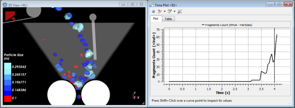
It is important to realize that breakage data is only collected after the Breakage Start value on the Solver | Time tab is reached. This is to allow enough time for the particle flow within your simulation to reach a steady state before breakage calculations begin.
For further details on the specific models, tips, and limitations see the About Particle Breakage topic.
Set up your simulation as you normally would (see also Set Simulation Parameters), ensuring all of the following:
During the Set Simulation-Wide Parameters step, on the Solver | Time tab, you have set the values you want for both Breakage Start and Breakage Delay after Release. (See also About Solver Parameters.) Tip: It is best practice to set your Breakage Start time to begin after a steady state has been reached for your particle flow.
During the Add and Edit Particle Sets step, you have done all of the following for each of the |Gloss7|s you want breakage enabled:
On the Particle tab, you have ensured that one of the following Shape | Composition option combinations are selected:
Either Straight or Custom Fiber Shape | Multiple Element Composition
Custom Shell Shape | Multiple Element Composition
Solid Polyhedron Shape | either Single Element or Multiple Element Composition
Solid Briquette Shape | Single Element Composition
Solid Faceted Cylinder Shape | Single Element Composition
Solid Custom Convex Polyhedron Shape | either Single Element or Multiple Element Composition
Solid Custom Concave Polyhedron Shape| Multiple Element Composition
If you have selected a Single Element particle set, you have done all of the following:
On the Particle | Breakage tab, you have selected the Enable Breakage checkbox.
From the Criteria sub-tab, you have selected the Instantaneous Breakage model you want from the Model list, and have defined its associated parameters.
From the Fragments sub-tab, you have entered the values you want under Limits, have chosen the model you want from the Distribution model list, and have defined its associated parameters.
If you have selected a Multiple Element particle set, you have done all of the following:
On the Particle | Breakage tab, you have selected the Discrete Breakage model you want from the Model list.
You have defined the model's associated parameters.
Process your simulation as you normally would. (See also About Starting a Simulation.)
After your simulation reaches as least as far as the Breakage Start time, do one or more of the following:
From a 3D View window (see also About 3D View Windows), observe the changes to the particle shapes as they fragment and break.
From the Data panel, select Particles and then from the Data Editors panel, select either the Properties or Curves tab and then create a plot (see also Graph Data within Rocky by Creating a Plot or Histogram) or visualize the resulting fragments-related Properties in a 3D View window (see also About 3D View Windows).
See Also:
(See also About Particle Assemblies.)
Begin setting up your simulation as you normally would (see also Set Simulation Parameters).
During the Add and Edit Particle Sets step, do the following:
For each part you want represented in your final Assembly shape, create an individual Particle set. (See also Add a New Particle Set.) Tip: Ensure your Particle set meets the specific criteria for Assembly parts. (Refer to the Assembly Particle Shape Limitations section of the Particle and Input Limitations topic for details.)
Create another new Particle set (see also Add a New Particle Set), select it, and then from the Data Editors panel, do the following:
From the main Particle tab, define the Shape as an Assembly.
From the Shape sub-tab, add a new definition row for each individual part you want to include, and define each's part's position, size scale, and rotation parameters. (See also About Adding and Editing Particle Sets.) Tip: Check your settings in the Particles Details window. (About Particles Details Windows.) Note: For Assembly shapes, the Particles Details 3D view shows the actual position of the part when the size type is Original Size Scale and it is set to 1 (which is the default setting).
Define the rest of the shape settings as you normally would for any other Particle set. (Define what parameters you want on the Size, Movement, and Orientation sub-tabs.) Important:At this point, Rocky will calculate the mass, area, and other properties for the (whole) Assembly particle based on the values you have defined for the Particle sets upon which the individual parts are based, and the size of the parts you have defined within the Assembly. These properties will be calculated accurately by Rocky as long as your individual parts do not overlap; otherwise, the accuracy of these Rocky-calculated properties cannot be guaranteed and you should consider defining them yourself by specifying Custom Properties.
(Optional) If your Assembly shape requires its parts to overlap, and you require accurate mass, area, and other properties for your Assembly particle, consider specifying Custom Properties for your assembly by doing the following:
From the CAD program with which you designed your ideal (Assembly) particle shape, note the Area, Volume, Mass, Geometric Center, Center of Mass, and other properties you want Rocky to use for your Assembly particle shape.
In Rocky, from your Assembly particle's Particle | Custom Properties tab, enable the Change Assembly Properties checkbox, and then enter the information you want Rocky to use. Tip: You can use the colored dots in the Particles Details window to preview where your Center of Mass (blue dot) and Geometric Center (yellow dot) are located.
Finish setting up your simulation, process it, and then analyze the results as you normally would.
See Also:
If you want to observe how particles are affected by temperature changes brought on by the heating or cooling of other items around it, you may set up your simulation to model thermal properties. Turning on Thermal Modeling enables you to simulate conductive heat transfer from particles to other particles, and from particles to boundaries. When used with CFD Coupling methods, it can also simulate convective heat transfer between particles and fluids. (See also Set or Modify Fluid and/or Air Flow Properties.)
Tip: For examples and walk-through tutorials of thermal modeling in action, review the following resources:
Set up your simulation as you normally would (see also Set Simulation Parameters), ensuring all of the following:
During the Set Simulation-Wide Parameters step, on the Physics tab, select the Enable Thermal checkbox. (See also About Physics Parameters.) Note: If you decide to enable Intra-particle Collision Statistics, know that the Temperature property will not be available to view on the Particles Details window, but can still be viewed from the main Particles entity or through a 3D View window. (Se also About Intra-Particle Collision Statistics.)
During the Add and Edit Geometry Components step, on the Geometry sub-tab for each of your wall components, set what you want for Thermal Boundary Type and Temperature.
During the Add and Edit Particle Sets step, on the Particle tab for the Particle set(s) you want affected by Thermal, ensure that on the Composition sub-tab for any particles you have you have selected Multiple Elements from the Composition list, that you also set the Conductivity Ratio parameter to the value you want.
During the Modify Material Properties step, on the Materials tab for each of your particle and/or boundary materials, set all of the following parameters:
Thermal Conductivity
Specific Heat
Poisson's ratio (See also About Modifying Material Compositions.)
During the Add and Edit Particle Inputs step, for each Particle Input, set the Temperature of each Particle set row. (See also About Adding and Editing Particle Inputs.)
If coupling your simulation with CFD methods, then during the Set or Modify Fluid and/or Air Flow Properties step, set what you want for the Convective Heat Transfer Law. (See also About Using the 1-Way Fluent Method, About Using the 2-Way Fluent Method, or About Using the 1-Way Constant Method). Note: If coupling your simulation with the 1-Way Constant method specifically, ensure you also set the values you want for constant Temperature, Thermal Conductivity, and Specific Heat. (See also About Using the 1-Way Constant Method.)
Process your simulation as you normally would. (See also About Starting a Simulation.)
Set up your simulation as you normally would (see also About SPH Parameters), ensuring all of the following:
During the Set Simulation-Wide Parameters step, on the Physics tab, select the Enable Thermal checkbox. (See also About Physics Parameters.) The Cleary model for thermal transfer is automatically selected.
During the Add and Edit Geometry Components step, on the Geometry sub-tab for each of your wall components, set what you want for Thermal Boundary Type and Temperature.
If you simulation also involves DEM particles: During the Add and Edit Particle Sets step, on the Particle tab for the Particle set(s) you want affected by Thermal, ensure that on the Composition sub-tab for any particles you have you have selected Multiple Elements from the Composition list, that you also set the Conductivity Ratio parameter to the value you want.
During the Modify Material Properties step, on the Materials tab set all of the following parameters for the fluid material:
Thermal Conductivity
Specific Heat
Process your simulation as you normally would. (See also About Starting a Simulation.)
Tip: When you are ready to analyze your simulation (see also Analyzing a Simulation), you might pay special attention to the following Properties (see also About Properties):
Temperature (for walls, conveyors, particles and fluids)
Specific Heat (only for fluids)
Thermal Conductivity (only for fluids)
See Also:
A 3D View of your simulation will always contain the Rocky logo but you can choose to add your own company logo to the view, too. This may be useful in cases where you are showing simulation images or animations to clients and want to brand your work.
You add a logo image by using the Overlay tab on the Window Editors panel. Logos are added as images and can be positioned anywhere on the 3D View window that you like.
Using separate image editing software, open the logo file you want to use and ensure the display size is appropriate.
Ensure your image is saved as either a PNG, JPG, BMP, or PNP file.
Open the simulation project to which you want to add the logo and select the 3D View window you want.
Using the Overlay tab on the Window Editors panel, add the logo to the 3D View as an Image Overlay. (See also Add or Edit an Image Overlay for a 3D View Window.)
See Also:
For projects where you have spent time and effort setting up several 3D View windows, Workspaces, and User Processes just the way you like, you can now export all of that setup criteria and reuse it in other projects. This is an alternative to recording or writing a script to do the setup for you, which requires you to know beforehand exactly how you want your views and processes to work. With this feature, you can decide after the fact whether you want to reuse the setup for another project or not.
This can be useful in cases where you have already run several similar simulations but your client suddenly wants to see new views or processes. By using this feature, you can set up the new views and processes in one project, and then apply those same views and processes to the rest of the projects in your set.
Rocky enables you to export this setup criteria to either a rocky_template file or to the clipboard, and even
lists each component that was exported in a separate dialog (Figure 1) for confirmation purposes.
 Example dialog that appears after exporting project context
In your new project, you can then choose to import the saved criteria from those same two locations.
Once imported, Rocky simply creates new 3D View windows, Workspaces, and User Processes to match what was exported. If you already have 3D View windows and User Processes in your project at the time of Import, Rocky will retain these items while adding the new ones to the project.
Ensure that your 3D View windows, Workspaces, and User Processes are set up the way you want.
From the File menu, point to Export project context and then do one of the following:
To ensure reuse of the project context for longer than just the immediate timeframe, select To file, and then do all of the following: a. From the Save project context dialog, select the location to which you want to save the
rocky_templatefile, name it in the File name box, and then click Save. b. In the Finished exporting context dialog, review the items listed, and then click OK.To reuse the project context for only the immediate timeframe, select To clipboard, and then in the Finished exporting context dialog, review the items listed, and then click OK.
The 3D Window, Workspace, and User Process setups are ready to import into another project.
Ensure the project that you want to apply the previously exported setups is open in Rocky.
From the File menu, point to Import project context and then do one of the following:
To import from a previously exported file, select From file, and then from the Restore project context dialog, locate and select the
rocky_templatefile you want to use, and then click Open.To import from the clipboard, select From clipboard.
The 3D Window, Workspace, and User Process setups you previously exported are added to the project.
See Also:
When setting up a new GPU card for use with Rocky, there are two steps you can take that might help make processing your simulations on GPU smoother and faster:
Turn off the Windows Timeout Detection and Recovery (TDR)
Enable double-precision processing
See below for specific instructions.
Application: This procedure is particularly useful when you have a single NVIDIA GPU card. But it can also be useful for any GPUs used by Rocky in general.
Symptom: Your Rocky simulations sporadically stop during the middle of a complex simulation, resulting in an incomplete calculation and an error (Figure 1). This is caused by Windows believing the GPU card is non-responsive because it is taking longer than expected to return an answer on a difficult calculation. Turning off TDR for your GPU allows the card the necessary time to execute the computation.
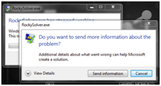
To turn off TDR for a GPU card:
Ensure that you have successfully installed your GPU card and associated drivers, and have restarted your computer.
Download and install the latest NVIDIA Nsight Visual Studio Edition from Nvidia.
 Figure 2: Installation confirmation screen for Nsight Visual Studio Edition
 Notes:
As seen in Figure 2 above, you will need only to install the Nsight Monitor option; the Nsight Visual Studio option is not necessary.
You may need to Subscribe as a developer (free of charge) on the Nvidia website, if you haven't done it before, in order to download the Nsight Visual Studio Edition (Figure 3).
 Figure 3: Subscribe to Nvidia developer program
 Restart your computer.
From the Windows Start menu, under NVIDIA Corporation, click Nsight Monitor (Figure 4).
 Figure 4 Nsight Monitor in Windows Start menu
A new Nsight Monitor icon appears in your Notification Area.
Figure 4 Nsight Monitor in Windows Start menu
A new Nsight Monitor icon appears in your Notification Area.From your Notification Area, right-click the Nsight Monitor icon and then select Options (Figure 5).
 Figure 5: Nsight Monitor in Notification Area
From the NVIDIA Nsight Options dialog, on the General tab, set WDDM TDR enabled to False (Figure 6).
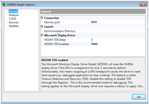 Figure 6: NVIDIA Nsight Options dialog
Click OK.
Restart your computer.
Application: You have one or more GPU cards from the NVIDIA Titan family.
Symptom: You are seeing slower than expected results on your Titan family GPU card. This could be a result of not yet enabling double-precision processing. Doing so will speed up certain Rocky calculations, thereby reducing your overall processing time, at the expense of slowing down your graphics visualization performance. Additionally, it has been found that a Titan card using double precision will take longer when simulating Spheres (~20%), but will be faster when simulating shaped particles (~200%).
To enable double-precision processing for your GPU cards:
Ensure that you have successfully installed your Titan card(s) and associated drivers, and have restarted your computer.
Right-click your Windows desktop, and then click NVIDIA Control Panel (Figure 7).
 Figure 7: Windows desktop right-click menu showing NVIDIA Control Panel option
In the NVIDIA Control Panel window, do all of the following:
From the Select a Task list, select Manage 3D settings.
In the Global Settings tab under Feature, select Double precision and then from the drop-down list, ensure all your Titan GPU cards are enabled (checked) (Figure 8).
 Figure 8: Manage 3D Settings section in the NVIDIA Control Panel
Click OK.
Restart your computer.
See Also:
Python is the programming language upon which Rocky is built. While knowing how to understand Python is not a requirement for using Rocky, there are several ways you can use the language to customize and extend the features included within the program.
For example, one way in which Python is useful is for creating and editing scripts. (See also Creating Your Scripts.)
You can also use Python to customize an Advanced Expression for a Property or Curve function. (See also About Customizing Properties or Curves.)
Rocky also includes a special panel that you can use to edit the underlying Python code and explore Rocky's API:PrePost functionality. To open this panel, from the Tools menu, click Python Shell.

Note: This version of Rocky supports only the Python 3 language. If your scripts were built using an older version of Rocky-or an older version of Python (for example, Python 2.7)-they might no longer work in this version. (See also My old script no longer works.)
Tips:
Find Rocky APIs quickly by using the Contents, Search, or Index tabs in the Rocky API:PrePost Manual. (From the Rocky Help menu, point to Manuals and then click API:PrePost Manual.)
View and modify sample scripts in the PrePost Scripts Repository section on the Rocky Customer Portal. (If you do not already have sign-in information for the customer portal, please contact your Rocky representative for assistance.)
See Also: