The linear elastic model is the default model for joints in Rocky. In this model, each force and moment is directly proportional to the corresponding linear or angular joint deformation:
(3–3) |
(3–4) |
(3–5) |
(3–6) |
(3–7) |
where:
and
are, respectively, the normal, the tangential, the torsional, and the two bending stiffnesses associated to the joint, defined below.
and
are, respectively, the normal and tangential relative displacements between the center points associated to the joint on the two connected elements.
,
and
are the torsional angle and the first and second bending angles, respectively, as defined in the previous sections. In the fiber case there is only one bending angle
, so Equation 3–7 is disregarded in that case.
The five stiffnesses present in the previous equations are calculated in Rocky using the following expressions:
(3–8) |
(3–9) |
(3–10) |
(3–11) |
(3–12) |
where:
and
are the normal and tangential stiffnesses per area unit, respectively, defined below.
,
,
and
are, respectively, the area, the polar second moment of area, and the two planar second moments of area of the cross section of the joint. In fibers, this cross section is a circle of the same diameter of the connected elements. If those elements are of different diameters, only the smaller diameter is used in the calculations. In shells, the cross section is a rectangle whose dimensions are the length of the corresponding triangle's edge and the shell thickness, respectively. In solid particles, the cross section is equal to the triangular face common to two tetrahedral elements connected by the joint.
,
,
and
are the values of the user-defined elastic ratios for each type of joint deformation: normal, tangential, torsion and bending, respectively. These values will be available for input in the Rocky UI only if the checkbox is enabled for the corresponding particle group. Otherwise, all four values will be equal to the value specified for , the only option available in that case. Allowed values for these parameters are in the range
for fibers, and
for any other particle.
For fibers and shells, the stiffnesses per area unit are computed using these expressions:
(3–13) |
(3–14) |
where:
is the Young's modulus attributed to the joint. In most cases, it will be considered equal to the Young's modulus specified for the particle's material. The only exception is the case of custom fibers, for which it can be calculated using described below.
is a characteristic length for the joint. For fibers, it is defined as the average length of the sphero-cylinder elements that make up a fiber. For shells, it is defined as
times the average length of the edges on the triangular mesh that defines the main geometry of the shell.
is the Poisson's ratio specified for the particle's material.
The Young's modulus attributed to the joints can be made non-uniform defining an extra
parameter for each segment in a custom fiber's centerline. This parameter is a Young's
modulus multiplier whose value can be specified at an optional column in the file defining
the fiber's geometry. For a joint between two elements with multipliers and
, respectively, the Young's modulus value will be computed as:
(3–15) |
where is the Young's modulus specified for the particle's material.
Solid flexible particles pose a special case in the determination of the elastic
properties for joints. In Rocky, these properties are determined using curves obtained
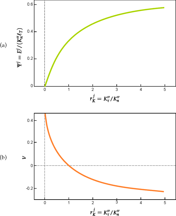
numerically by Potapov & Campbell. Those curves, reproduced in Figure 3.9: (a) Dimensionless Young's modulus and (b) Poisson's
ratio as a function of the stiffness ratio for composite
bodies formed by Delaunay tetrahedra. Extracted from Potapov
& Campbell (1996)., relate the dimensionless Young's modulus and the Poisson's ratio
with the joint stiffness ratio
, respectively.
The joint stiffness ratio is defined as:
(3–16) |
Figure 3.9: (a) Dimensionless Young's modulus and (b) Poisson's ratio as a function of the stiffness ratio for composite bodies formed by Delaunay tetrahedra. Extracted from Potapov & Campbell (1996).

The dimensionless Young's modulus is defined here as:
(3–17) |
where is the characteristic length of the particle's tessellation, which in
Rocky is considered equal to the average length of the edges of all tetrahedral elements
that make up the particle.
In order to determine values of and
using the Potapov & Campbell curves, the following procedure is
considered:
Considering
, the value of the Poisson's ratio of the particle's material, the value of the stiffness ratio
is determined as the corresponding abscissa in curve (b) of Figure 3.9: (a) Dimensionless Young's modulus and (b) Poisson's ratio as a function of the stiffness ratio for composite bodies formed by Delaunay tetrahedra. Extracted from Potapov & Campbell (1996)..
That value of
is then used to determine the corresponding value of the dimensionless Young's modulus
from curve (a) in Figure 3.9: (a) Dimensionless Young's modulus and (b) Poisson's ratio as a function of the stiffness ratio for composite bodies formed by Delaunay tetrahedra. Extracted from Potapov & Campbell (1996)..
The corresponding value of
for the joint is determined using Equation 3–17.
Finally, the value of
is determined using Equation 3–16
The viscous damping model for joints is not a model that can be used alone, but it complements other joint models in order to add or increase energy dissipation. For instance, the linear elastic model described in the previous section does not include any energy dissipation mechanism by itself. Therefore, when used in isolation, it can produce simulations in which the elements of flexible particles may oscillate endlessly, even after the action of all external forces ceases. In order to overcome that situation, joint viscous forces and moments can be added through this model, that will dissipate energy and will reduce internal oscillations in flexible particles.
The joint viscous forces and moments in Rocky are defined, respectively, as:
(3–18) |
(3–19) |
(3–20) |
(3–21) |
(3–22) |
where:
and
are, respectively, the normal, the tangential, the torsional, and the two bending damping coefficients associated to the joint, defined below.
and
are, respectively, the normal and tangential relative velocities between the center points associated to the joint on the two connected elements. The absolute velocity at each center point is the sum of the velocity of the element's center of mass and the tangential velocity due the rotation of the element around that center of mass.
,
and
are the three scalar components of the relative angular velocity between the connected elements. The axes associated to those components are the same axes considered in the decomposition of the angular deformations.
The normal and tangential damping coefficients for the joint are determined, respectively, using the expressions:
(3–23) |
(3–24) |
where:
is a user input parameter listed as Damping Ratio | Joint in the Rocky UI. Allowed values are in the [0, 1] interval. The higher the value of
, the faster must be the decay of oscillations.
is the effective mass of the joint, which is determined with Equation 2–10, considering the masses of the two connected elements.
Finally, the damping coefficients for the angular movements are calculated using the expressions:
(3–25) |
(3–26) |
(3–27) |
where ,
,
and
are, respectively, the area, the polar second moment of area, and the two
planar second moments of area of the cross section of the joint.
In order to enable the viscous damping model, it is only necessary to specify a value of the damping ratio larger than zero. Although this model was introduced in Rocky as a complement to the linear elastic model, it can be used with any other joint model, as a mechanism of additional energy dissipation.
Since Rocky v4.3, the bilinear elastoplastic model is included as a joint model option in Rocky, in order to simulate the behavior of flexible particles that may suffer permanent deformations when submitted to large external forces. This model may be especially useful for the simulation of industrial and agricultural fibers, although it can be applied also in Rocky to flexible shells. Only angular deformations are considered in the implementation of this model in Rocky, since usually they are more significant than axial tensile or compression deformations on the dynamics of fibers, especially bending.
Considering any of the angular directions, the basic relationship between the joint
moment and the angular deformation
according to the bilinear elastoplastic model can be written as:
(3–28) |
where:
is the joint stiffness in the purely elastic regime. Its value will be given by either Equation 3–10, Equation 3–11 or Equation 3–12, depending on the deformation direction being considered.
is the joint stiffness in the elastoplastic regime, computed with below.
is the threshold angle that marks the end of the purely elastic regime and the beginning of the elastoplastic regime, during the loading phase. This is an input parameter of the model that is listed in the Rocky UI as either or , depending on which deformation direction is being considered.
The value of the stiffness in the elastoplastic regime is related to the value on the purely elastic regime, through the expression:
(3–29) |
where is a model parameter listed in the Rocky UI as . Admissible values for
this parameter are in the [0, 1] interval. In the limit
, the model will behave as a elastic-perfectly plastic model, while in the
other end,
, there would not be change of regime at all and the model would reduce to
the linear elastic model. For any other intermediate value of the plastic ratio, the
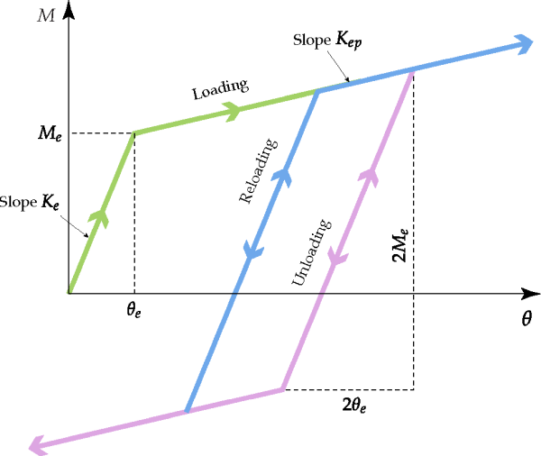
response of the model will be as the green line in Figure 3.10: Typical loading-unloading-reloading cycle for the bilinear elastoplastic model in
Rocky. , with a
sudden reduction of slope at
.
Figure 3.10: Typical loading-unloading-reloading cycle for the bilinear elastoplastic model in Rocky.

If at any point during the elastoplastic regime the angular deformation begins to
diminish, the unloading trajectory will follow a different path from the loading. The
unloading path will have initially the same slope of the purely elastic regime, as illustrated by the purple line in Figure 3.10: Typical loading-unloading-reloading cycle for the bilinear elastoplastic model in
Rocky.. If during the unloading the angle is reduced a value larger than
, the path will change the slope again to
, the one defined for the elastoplastic regime. Any reloading initiated
during this regime will follow a path like the blue line in Figure 3.10: Typical loading-unloading-reloading cycle for the bilinear elastoplastic model in
Rocky.
. Again, the path begins with a slope equal to
, as in the elastic regime, until it switches to
when the angle variation is equal to
. If at any point of a line with slope
the angle variation is reversed, the new path will preserve the slope,
only the orientation will be the opposite. The cycle described here follows the kinematic
hardening rule.
An additional option available for the bilinear elastoplastic model is a sudden
reduction on the moment value, when the angular deformation reaches the threshold value , in addition to the change on the stiffness value. This model feature
may represent an instantaneous reduction in the resistance capacity of the joint to
angular deformations, due to material failure.
This option is activated when the checkbox With Failure is
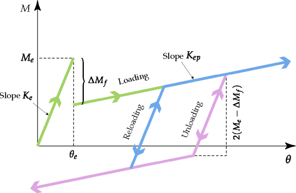
turned on in the Rocky UI. The effect of this feature can be seen on the diagram of ,
where the value of the moment has a reduction of the first time the angular deformation attains the value
during loading. The magnitude of the moment reduction is given by:
(3–30) |
where is a model parameter listed in the Rocky UI as Failure
Ratio, which accepts values in the [0, 1] interval. A zero value for this
parameter means no moment reduction at all, while
will imply a reduction to zero in the resistance capacity of the joint.
Figure 3.11: Cycle of loading-unloading-reloading for the bilinear elastoplastic model with failure.

Figure 3.11: Cycle of loading-unloading-reloading for the bilinear elastoplastic model with failure. shows an example of a cycle of deformation when
the failure option is enabled for the bilinear elastoplastic model. After the failure
moment reduction, the behavior of the paths of unloading and reloading is similar to the
ones described for the cycle without failure. The difference is in the extension of the
portion with slope on the unloading and reloading paths. As depicted in , there will be a
change to a slope
when the variation on the moment will reach a value equal to
.


